Geometrodynamical Analysis to Characterize the Dynamics and Stability of a Molecular System through the Boundary of the Hill’s Region ()
1. Introduction
The phase space structure for the vibrational dynamics of molecular systems with strong chaotic behavior is a very interesting topic in chemical processes [1] .
For practical applications several chaos indicators are used in literature, such as maximun Lyapunov exponent (LE) [2] , fast Lyapunov indicator [3] [4] , frequency map analysis [5] , small alignment index (SALI) [6] [7] , or the stability geometrical indicator (SGI) [8] .
In this paper we study the nonlinear Hamiltonian dynamics and stability of the vibrational dynamics of the isomerizing LiNC/LiCN molecular system [9] -[15] from a geometrodynamical perspective using the SGI indicator, by rewriting the dynamics in a geometric language, where a Riemannian manifold is defined by adding a particular metric to the corresponding configuration space. To this end different metrics are used in literature. Among them, the Eisenhart [16] , Finsler [17] , Horwitz [18] -[21] or Jacobi [22] -[29] are worth mentioning. We consider the Jacobi metric obtained from the Maupertuis’ Principle (1744), where geodesics [30] [31] (natural motions) are identified with trajectories of the system, and the stability can be analyzed through the study of the curvature of this Riemannian manifold via the Jacobi-Levi-Civita equations (JLC) [31] . Once the dynamical system is geometrized, physical magnitudes can be identified with geometrical ones, as indicated in Table1
This approach has been applied successfully in the calculation of Lyapunov exponents in Hamiltonian systems with many degrees of freedom [25] , after simplifying the JLC equations by coarse graining. We can define via the JLC equations the SGI indicator along trajectories. This indicator has been recently used to study the stability of trajectories in this molecular system [8] . We will use SGI for short times to locate stable periodic trajectories (with its corresponding chains of islands) and chaotic ones as local minima or maxima respectively of this indicator.
The boundary of the Hill’s region1 for systems with Gaussian curvature everywhere positive (locally stable) has been considered as a very important set to generate unstabilities because of its curvature [32] . As in the classical billiard problem non convex points (negative curvature) of the boundary are considered defocusing points related with unstable behavior of trajectories reaching these points. Thus trajectories probing the non convex points of the boundary are always chaotic and those trajectories reaching uniquely convex points of the boundary are regular as indicated in [32] . In this paper we show that this statement is not true in general showing that although our system is positively curved everywhere we can locate chaotic trajectories restricted to convex parts of the boundary of the Hill’s region and regular trajectories reaching non convex points.
The organization of the paper is as follows. In Sections 2 and 3 the geometric approach is described, relating chaos with JLC equations. In Section 4 the model LiNC/LiCN and its geometrization are presented. In Section 5 we present the results for trajectories with initial conditions at the boundary of the Hill’s region using the SGI. In Section 6 the importance of the boundary in order to study the stability of trajectories is discussed. Finally, the conclusions are summarized in Section 7.
2. Geometrodynamical Perspective
We consider the conservative system described by the Lagrangian2
 (1.1)
(1.1)

Table 1. Equivalence between some relevant magnitudes in the Dynamical and Geometrical views of the Classical Mechanics.
with  the kinetic energy tensor and
 , defined in the domain of the configuration space
 . We can make the following identification

being  the conjugate momenta in the phase space
 .
.
The Hamilton’s principle of least action can be connected with the Maupertuis’ principle which establishes as the natural motions those whose asynchronous trajectories with fixed end points are extrema for the action integral , i.e.
  with
with
 (1.2)
(1.2)
where  is the kinetic energy and
  the total energy (conserved)

being  the differential of length3. So the trajectories for the system corresponds to geodesics for the Riemannian manifold endowed with the metric that in coordinates can be written as
 (1.3)
(1.3)
called Jacobi metric. The configuration space for the system is the previous Riemannian manifold 
where  represent the local coordinates and
  being referred to as mechanical manifold. It can be shown that the trajectory followed by a particle affected by the potential energy function
  in the Euclidean space is equivalent to the motion of a free particle in the restricted mechanical manifold
 . Thus there is a correspondence between dynamics in an Euclidean space (zero curvature) and kinematics in a Riemannian manifold.
Geodesics are autoparallel curves, so they are described through these equations

with  the affine connection compatible with the metric, in coordinates
 (1.4)
(1.4)
and  the Christoffel symbols from the metric
 , which are calculated as
 (1.5)
(1.5)
Changing ds by dt

in Equation (1.4), we get
 (1.6)
(1.6)
that corresponds to trajectories parametrized by physical time .
.
3. Curvature and Chaos. Jacobi-Levi-Civita Equations (JLC)
The sectional curvature ,
,  at the point
  and tangent plane
  on the Riemannian manifold
  at this point (Gaussian curvature in dimension two), determines the velocity of spreading for the geodesics starting at
  tangent to
 .
.
The evolution for this geodesic deviation obeys the JLC equations
 (1.7)
(1.7)
with  geodesic in
 ,
,  the covariant derivative along the curve
  and
and
 the Riemann-Christoffel curvature tensor [30] .
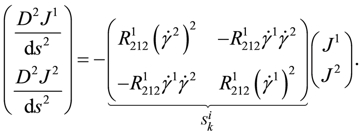
In our case,  and
and  the geodesic deviation vector field along the fiducial trajectory
 then
then
 (1.8)
(1.8)
with  the stability tensor, in a local chart
  and
and 
 (1.9)
(1.9)
The matrix  is symmetric and defines a selfadjoint mapping
  relative to
  as
as 
where , in a local chart
  and
and  can be expressed as
and the associated quadratic form 

with  the inner product, that can be diagonalized by solving

with eigenvalues  and
and , and the corresponding eigenvectors
  and
and
 being mutually orthogonal. These eigenvectors when normalized define a convenient basis
  obtaining the new convenient moving frame in terms of the canonical local chart of
  as follows
 (1.10)
The equations (1.7) can be easily expressed in this basis being parallel transported along  solving the dynamical equations
 (1.11)
with  we solve (1.11) using the Taylor expansion
 . (1.12)
If the vector field  is expressed as
  we can write (1.9)
 (1.13)
with  the scalar curvature for metric
 . The evolution for
  is as much lineal and the stability is determined by the scalar
  (from now on referred as
 ) along the fiducial curve.
Fixing a constant length  for the trajectory, we define the dynamical magnitude Stability Geometric Indicator (SGI) as
 (1.14)
with initial conditions . We will use this indicator to compare the mutual relative stabilities for different trajectories.
4. Isomerization System LiNC/LiCN
4.1. The Model
We study the two degrees of freedom model for the isomerizing molecular system LiNC/LiCN, where the bond NC is kept frozen at its equilibrium distance  a.u. Studying the problem in the phase space, the classical vibrational (with zero total angular momentum) Hamiltonian for the dynamical system in Jacobi coordinates is given by
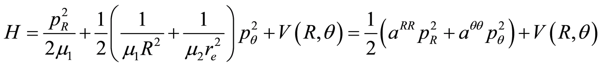 (1.15)
where  is the distance from the Li atom to the NC center of mass,
  is the NC distance,
  is the angle defined by the R and CN vectors,
  and
and  are the corresponding conjugate momenta, and
and  represent the Li-NC and NC reduced masses, respectively.
The potential energy surface  is defined by an expansion in Legendre polynomials

where parameters  are taken from the literature [33] . As can be seen in Figure 1 it presents two potential wells (elliptic points), corresponding each one to a stable isomer with linear configuration: LiCN where
  a.u.,
a.u.,  rad and
  and LiNC where
  a.u.,
a.u., 
rad and  and a saddle point (hyperbolic point) at
  a.u.,
a.u.,  rad and
 . The minimun energy path (MEP) connecting the two isomer wells has been plotted as a dashed line superimposed to the potential energy surface in Figure 1. It can be written as the following Fourier expansion:

Figure 1. (Left) Potential energy surface for the LiNC/LiCN isomerizing system. Contours lines have been plotted every . The minimum energy path connecting the two isomers is shown as a dashed line. (Right) Energy profile along the minimum energy path.

The energy profile associated to the MEP is given in the right panel of Figure 1.
The dynamics is monitored by PSOS (Poincaré surface of section). In order to obtain the most complete dynamical information we compute them taking the minimun energy path,  , as the sectioning plane [34] . This PSOS is made an area preserving map defining a new set of canonical variables
  as:
as:

Now the PSOS is defined by the condition  and
and  is obtained from the Hamiltonian conservation
 corresponding to the negative branch in the calculation of the second-order equation obtained. We represent PSOS values in the interval
  rad taking into account the symmetry of the molecular system.
4.2. Jacobi Metric
Considering the Hamiltonian of the system (1.15) then4
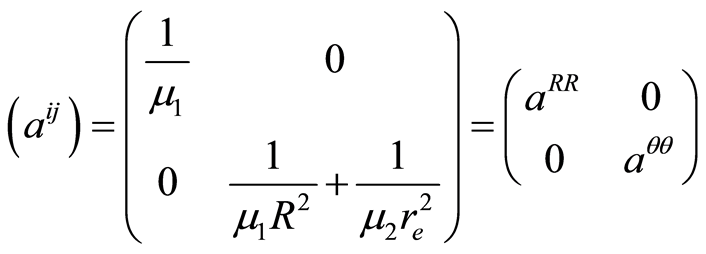
and the Riemannian manifold  is given by
  and
and

 (1.16)
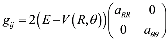 . (1.17)
The Christoffel symbols for the metric (1.17) are calculated using (1.5), obtaining
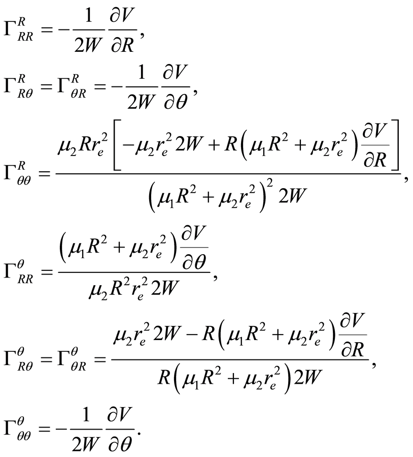 (1.18)
Trajectories parametrized by physical time  are calculated integrating the equations (1.6) after replacing the corresponding values of
  (1.18)
 (1.19)
4.3. Jacobi-Levi-Civita (JLC) Equations
Geodesic deviation vector field  with
with  along the fiducial trajectory
is used in the JLC equation (1.7). Rewriting equation (1.13) for physical time  we obtain
 (1.20)
where the scalar curvature  for the metric
  determines the local stability for geodesics around the fiducial one at
 . If
. If  is the dimension of the system it can be written as
 (1.21)
with  the scalar curvature for the space and
  the Laplace-Beltrami operator both for metric
 , in our case for
 (1.22)
 (1.23)
with  the Christoffel symbols of the metric
 ,
,
 (1.24)
replacing (1.24) in (1.23)
 (1.25)
 (1.26)
The expression for the curvature (1.22) of the mechanical manifold  needed for solving Equation (1.20) is

This scalar curvature (Gaussian curvature) is everywhere positive, i.e. every trajectory is locally stable. The differential equations system to integrate numerically consists on (1.19) and (1.20) simultaneously.
5. Locating Stable and Chaotic Trajectories with SGI at the Boundary of the Hill’s Region
In order to characterize the dynamics of the system the selection of initial conditions to integrate trajectories is very important. All the trajectories we have integrated reach the boundary of the Hill’s region at some time. This fact motivate to study the dynamics in our molecular system through trajectories with initial conditions at this boundary.
We have calculated the value of SGI for short times of trajectories with initial conditions  all along the boundary
  i.e.
i.e.  and
and  (kinetic energy equals zero) with a value for energy
 . Equation (1.22) is singular at these points so the calculations have been done for an energy
 lightly higher with value
  obtaining the results plotted in Figure 2.
Stable trajectories and chaotic ones for the interval  rad for the upper region of the boundary (red colour in upper left graph in Figure 2) are represented in Figure 3 labeled from (1) to (8).
The stable periodic trajectories correspond with local minima values of SGI in particular the points (1), (2), (3), (5) and (7), and the chaotic trajectories with (4) and (8). The trajectory represented with (7) is the most stable trajectory of the system related with the KAM torus with the most irrational relation of frequencies, being this torus the last one broken in the transition from order to chaos. The corresponding trajectories in  are represented in the upper graphs of Figure 3.
Chain of islands are represented as those forming the corresponding valleys in the global SGI diagram, the stability of the resonant periodic orbit in the minimun is indicated by the width of the valley as illustrated in the Poincaré Sections in Figure 4.
In order to locate a chaotic trajectory from the global SGI diagram we search for hyperbolic points located between the chains of islands (Poincaré Birkchoff Theorem) so we take initial conditions at the extrema of the previous valleys represented by local maxima labeled by (4) and (8) in Figure 3. The Poincaré sections for all these trajectories are illustrated in Figure 4.
The indicator SGI is calculated along trajectories with initial conditions at the boundary for energy  locating a chaotic trajectory and a periodic one represented by the maximum and minimum points in the graph for SGI in Figure 5. The Poincaré sections are illustrated in Figure 6.

Figure 2. Values of SGI for different trajectories with initial conditions all along the boundary of the Hill’s region (upper left graph) for the energy,  , the interval
  rad of the upper region (red) is zoomed where a stable periodic trajectory (i) and another from the chain of islands (ii) are marked.
6. SGI and the Curvature of the Boundary of the Hill’s Region
The boundary of the Hill’s region and particularly the sign of its curvature is often related with the stability of trajectories bouncing on it. In systems with Gaussian curvature everywhere positive inside the Hill’s region is quite natural consider the non convex (negative curvature) regions of the boundary as source of unstabilities for trajectories bouncing on it. In this sense we could say that regular trajectories should probe or touch only convex regions (positive curvature) of the boundary of the Hill’s region as well as chaotic trajectories should probe the non convex region at least once [32] .
We show that this statement is not true in general finding a stable periodic trajectory bouncing on non convex

Figure 4. Poincaré sections for all trajectories represented in Figure 2 and Figure 3 for the energy . The black curve represents the boundary of the accessible region in the phase space.
region (negative curvature) of the boundary and another chaotic trajectory restricted to convex regions of this boundary.
The curvature  of the boundary of the Hill’s region considered as the set level
  can be calculated

We study the convexity for different set levels  and plot the points of curvature zero (change of convexity) as the red curve in Figure 7, the non convex points on the lower region of the boundary for the energy
  are in the interval
  rad.
rad.
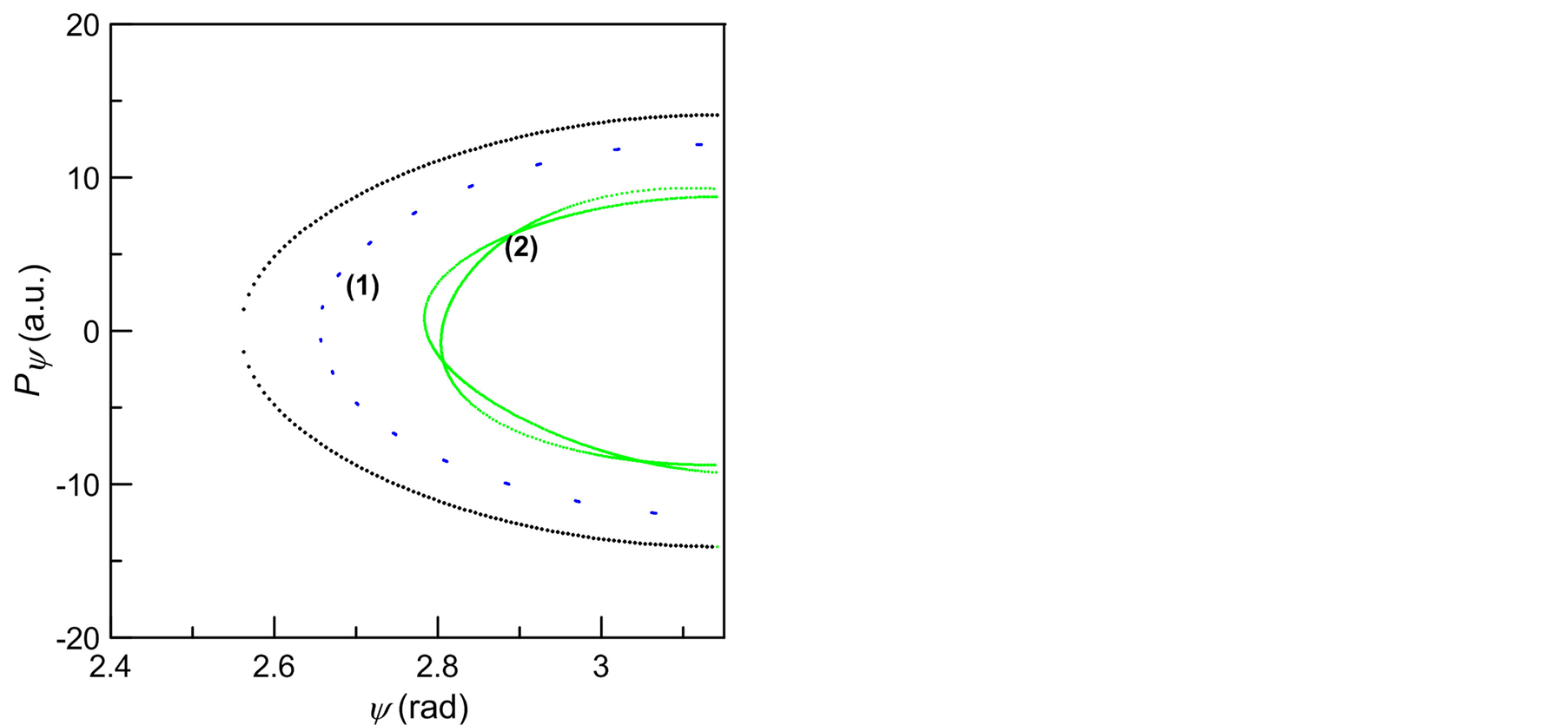
Figure 6. Poincaré sections for the two trajectories represented in Figure 5 at the energy . The black curve represents the boundary of the accessible region in the phase space.

Figure 7. A chaotic trajectory (a) restricted to convex points of the boundary of the Hill’s region and a stable periodic trajectory (b) reaching the boundary at non convex points at the energy . These trajectories correspond to (4) and (i) respectively in Figure 4.
The two trajectories studied with this energy are labeled as (i) (regular) and (4) (chaotic) in Figure 4 where their corresponding Poincaré sections are plotted. These two trajectories in  and the zero curvature for the corresponding set level are plotted in Figure 7. The chaotic trajectory only probes the convex region of the boundary while the regular one bounces non convex points.
The behavior of the chaotic trajectory comes to support the well known idea of the parametric resonance as fundamental reason for the onset of chaos. But the regular trajectory motivates the idea of an additional stabilization mechanism.
When defining the Jacobi metric  is quite often to understand the potential energy as curving the underlying space (with the kinetic energy tensor
  as metric), in the particular case of an underlying space of curvature zero (usually
 ) the first term in the right hand side of Equation (1.22) is zero and the curvature is caused by the energy potential. In our molecular system the kinetic energy tensor
  defines an underlying space positively curved with curvature
  expressed in (1.26). Thus although the potential energy is removed the space is equally positively curved.
Taking into account the stability is ruled by (JLC) Equations (1.13) where  includes the underlying curvature
  we can deduce the corresponding stabilization effect in the dynamics.
7. Conclusions
In this work, we have studied the vibrational dynamics of the isomerizing LiNC/LiCN molecular system described by a two-dimensional Hamiltonian model including a realistic potential function from a geometrodynamical perspective.
We have considered trajectories starting at the boundary of the Hill’s region and characterized the corresponding dynamics. Once defined the geometrical SGI indicator, we have calculated its value for short times along trajectories with initial conditions in the boundary of the Hill’s region, identifying stable periodic trajectories as local minima of that indicator and the width of the corresponding valley as measure of their stability. We have also identified chaotic trajectories as local maxima around the previous valleys just in the extrema of the corresponding stability region.
The importance of the curvature of the Hill’s region for the stability of trajectories has also been studied. We have found that stable trajectories for our system are mainly located at values of  rad and
  rad in the interval
 , corresponding to the most convex regions of this boundary. In pinciple, this would support the possibility of reducing our system to a classical billiard problem. However, we found a stable periodic trajectory out of this region. This stable periodic trajectory probes non convex points of the Hill’s region. On the other hand we also find a chaotic trajectory inside the supposed “stability region” bouncing uniquely on convex points of the boundary. Accordingly, the study of stability of trajectories in our molecular system cannot be reduced to a classical billiard problem, despite the Gaussian curvature everywhere positive inside the Hill’s region. This result comes to support the hypothesis of the parametric resonance as the main criterion for the onset of chaos in the case of the chaotic trajectories. However, in the case of the regular trajectories by probing non convex regions of the boundary we understand the underlying curvature
  (Equation (1.26)) to be the responsible for this lack of unstable behavior. This stabilization mechanism, through the scalar curvature of the underlying space, is currently being under active research in our group.
Acknowledgements
This research was supported by the Ministry of Economy and Competitiveness-Spain under Contracts No. MTM2012-39101 and ICMAT Severo Ochoa SEV-2011-0087.
NOTES
1Projection of the accessible region in the configuration space on the position coordinates.
2We will use the Einstein’s summation convention for repeated indexes, so 

3

4 , i.e.
  is the inverse matrix of
 .
.