A Study on the Performance of Absorbing Boundaries Using Dashpot ()
1. Introduction
A rational approach in the analytic study of various dynamic problems is to consider the wave propagation in infinite or semi-infinite media. However, it is practically impossible to find a closed form solution because of the complicated shapes involved in most of these problems. Therefore, the need is to apply a numerical method using the boundary element method (BEM), the finite element method (FEM) or a combination of these methods. Since FEM uses the original governing equations of motion in all the discretized subdomains, it is possible to observe directly all kinds of important phenomena like the mode transformation at the discontinuous interfaces. However, when an infinite domain is modeled by finite discrete subdomains, the wave happens to reflect after having reached the finite boundary of the relevant subdomain, which in turn influences significantly the response of the whole structural system. Accordingly, artificial boundary elements are necessary to annihilate the effect of the reflected wave caused by the discretization of the infinite domain. Such artificial boundary element is called absorbing boundary and is widely applied in wave propagation problems. To date, numerous boundary elements have been proposed by several researchers [1] -[8] . Among them, the absorbing boundaries proposed by Lysmer-Kuhlemeyer [1] and White et al. [4] can be easily applied in FEM programs since they reproduce the absorbing effect by means of viscous dampers or dashpots attached to the boundary of the element. However, it is still necessary to evaluate the performance of the absorbing boundary with regard to diverse types of loads to achieve numerical analysis applying absorbing boundaries to solve engineering problems.
This study intends to examine the performance of absorbing boundaries using dashpots for periodic loads at the surface. First, the performance of absorbing boundaries using dashpot is investigated by adopting the solution of Miller and Pursey [9] for the wave equation of a periodic load applied on the free surface. Then, the absorption ratios are computed by finite element analysis.
2. Wave Equation under Periodic Loading
This study examines the performance of the absorbing boundary using dashpot by means of analytical and numerical methods. The analytic method proceeds by introducing directly the absorbing boundary in the wave equation for the periodic load at the free surface. To that goal, the wave equation must be modified.
The wave equation of the semi-infinite domain subjected to periodic loading applied perpendicularly to the free surface can be expressed by Equations (1) and (2).
 (1)
(1)
 (2)
(2)
where  is as follows:
 (3)
(3)
In order to use Equations (1) and (2), the normalized wave number k must be decomposed into the wave number k1 in the x-direction and the wave number k2 in the y-direction because this decomposition is insensitive to the effect of the forced frequency when substituting directly Equations (1) and (2) in the absorbing boundary explained in Chapter 3.
 (4)
(4)
 (5)
(5)
where  is as follows.
 (6)
(6)
Equations (4) and (5) are the equations where the normalized wave number k is decoupled into k1 in the x-direction and k2 in the y-direction after mathematical computation.
3. Analytical Evaluation of Absorbing Boundaries
Equations (7) and (8) describe the absorbing boundary in which Lysmer-Kuhlemeyer [1] suggested a = b = 1 for the coefficients a and b, and White et al. [4] proposed the values arranged in Table1 Figure 1 represents Equations (7) and (8) on the boundaries.

Table 1. Values of absorbing boundary coefficients (White et al., 1977).

Figure 1. Absorbing boundary conditions.
 (7)
(7)
 (8)
(8)
The introduction of the two-dimensional harmonic wave Equations (9) and (10) in Equations (7) and (8) leads to Equations (11) and (12).
 (9)
(9)
 (10)
(10)
 (11)
(11)
 (12)
(12)
If a = b = 1, the value q = 0 satisfies simultaneously Equations (11) and (12) for arbitrary values of l and m. This means that, when q = 0 that is, when the wave attacks the boundary perpendicularly, the Lysmer-Kuhlemeyer absorbing boundary is perfectly satisfied. To that goal, Equations (7) and (8) are converted in polar coordinates. Here, the wave can have an angle of incidence perpendicular to the boundary if the wave Equations (4) and (5) in which the periodic load is expressed in polar coordinates is introduced.
The absorbing boundary conditions in polar coordinates are expressed in Equations (13) and (14).
 (13)
(13)
 (14)
(14)
For the analytical evaluation of the absorbing boundary conditions, the computed values of the left-hand side (LHS) and right-hand side (RHS) terms of Equations (13) and (14) are compared after substitution of Equations (4) and (5) in Equations (13) and (14). Here, since actual derivation is complicated, the partial derivatives of uR and u are computed using the numerical analysis program MATLAB and introduced in Equations (13) and (14) to obtain the values of the LHS and RHS terms with respect to R and q. The physical properties of the considered medium and the forced frequency are arranged in Table2
Figure 2 and Figure 3 plot the values of the LHS and RHS terms of Equations (13) and (14) in function of the distance R when q = p/4. The abscissa is the distance R (1 km £ R £ 100 km) and the ordinate represents the values of the LHS and RHS terms.
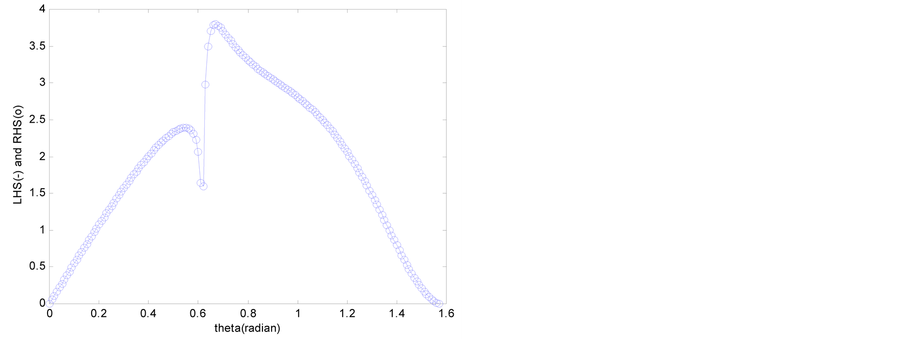
Figure 4 and Figure 5 plot the values of the LHS and RHS terms of Equations (13) and (14) in function of the angle of incidence q when R = 10,000 km. The abscissa is the angle of incidence q (0 £ q £ p/2) and the ordinate represents the values of the LHS and RHS terms.
In Figure 2 and Figure 3, the graphs of the Lysmer-Kuhlemeyer boundary are seen to coincide after approximately 30 km and 20 km, respectively. This is due to the fact that Equations (4) and (5) are asymptotic solutions obtained by the steepest-descent method after 1 wavelength of P and S waves. The graphs of the LHS and RHS are shown to coincide in Figure 4 and Figure 5, and indicate that the Lysmer-Kuhlemeyer absorbing boundary develops perfect performance with regard to the wave equation for periodic loading on the free surface.
Table 2. Physical properties of medium amd forced frequency.
 (a)
(a)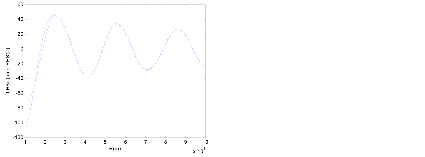 (b)
(b)
Figure 2. Values of LHS and RHS of Equation (13) (θ = π/4). (a) Lysmer-Kuhlemeyer; (b) White et al.
 (a)
(a) (b)
(b)
Figure 3. Values of LHS and RHS of Equation (14) (θ = π/4). (a) Lysmer-Kuhlemeyer; (b) White et al.
 (a)
(a) (b)
(b)
Figure 4. Values of LHS and RHS of Equation (13) (R = 10,000 km). (a) Lysmer-Kuhlemeyer; (b) White et al.
 (a)
(a)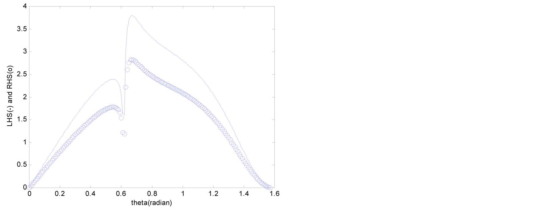 (b)
(b)
Figure 5. Values of LHS and RHS of Equation (14) (R = 10,000 km). (a) Lysmer-Kuhlemeyer; (b) White et al.
The boundaries of White et al. coincide in Figure 2 and Figure 4 but are different in Figure 3 and Figure 5. Similar results can be obtained even when changing the Poisson’s ratio, which indicate that the boundaries of White et al. cannot fulfill perfect performance against S waves. This can be attributed to the computational process of the absorbing boundary coefficient of Table1 Further examination should be carried out on this topic but will not be done in this paper since the present study focuses on the evaluation of the performance of absorbing boundaries using dashpot.
4. Numerical Evaluation of Absorbing Boundaries
Figure 6 to Figure 7 present the analytic model and load applied for the numerical analysis of this study. In Figure 6(a), the boundaries are modeled as semicircles to make the wave attack all the boundaries perpendicularly. The rectangular boundaries in Figure 6(b) are considered to examine the performance of the absorbing boundaries for waves presenting inclined angles of incidence. In Figure 6(a) and Figure 6(b), dashpots are installed on the boundaries to prevent the occurrence of reflected waves and absorb the waves so as to simulate infinite domains.
Figure 8(a) and Figure 8(b) display the layout of the receivers at which the displacements will be compared for evaluating the performance of the absorbing boundaries. In Figure 8(a) and Figure 8(b), Model A is considered to obtain the displacement without reflected wave. Here, the displacement is obtained by conducting the analysis until before the reflected wave generated at the boundary reaches the receivers in order to remove the
 (a)
(a) (b)
(b)
Figure 6. Analytic models. (a) Circular boundary; (b) Rectangular boundary.
 (a)
(a) (b)
(b)
Figure 8. Layout of receivers in absorbing boundaries. (a) Circular boundary model; (b) Rectangular boundary model.
effect of the reflected wave. Beside, Model B corresponds to the absorbing boundaries on which dashpots are attached. For this model, analysis is performed for a duration identical to Model A so as to measure the reflected wave generated at the boundary.
Figure 9 and Figure 10 plot the displacement in the x-direction according to the position of the receivers displayed in Figure 8.
In Figure 9 and Figure 10, the displacement of Model B without absorbing boundaries is completely different from that of Model A in which the reflected waves do not reach the receivers. On the other hand, the displacement of Model B applying the absorbing boundaries tends to coincide with that of Model A. Table 3 arranges the absorption ratios for the displacements in the xand y-directions according to the positions of the receivers in Figure 8(a). Here, q is the counterclockwise angle measured from the y-axis.
Table 4 arranges the absorption ratios for the displacements in the xand y-directions according to the positions of the receivers in Figure 8(b). Here, q is the counterclockwise angle measured from the y-axis.
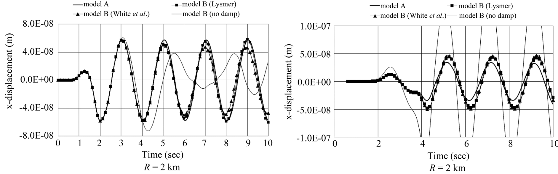
Figure 9. Displacement in x-direction at free surface receiver for circular boundary model of Figure 8(a).
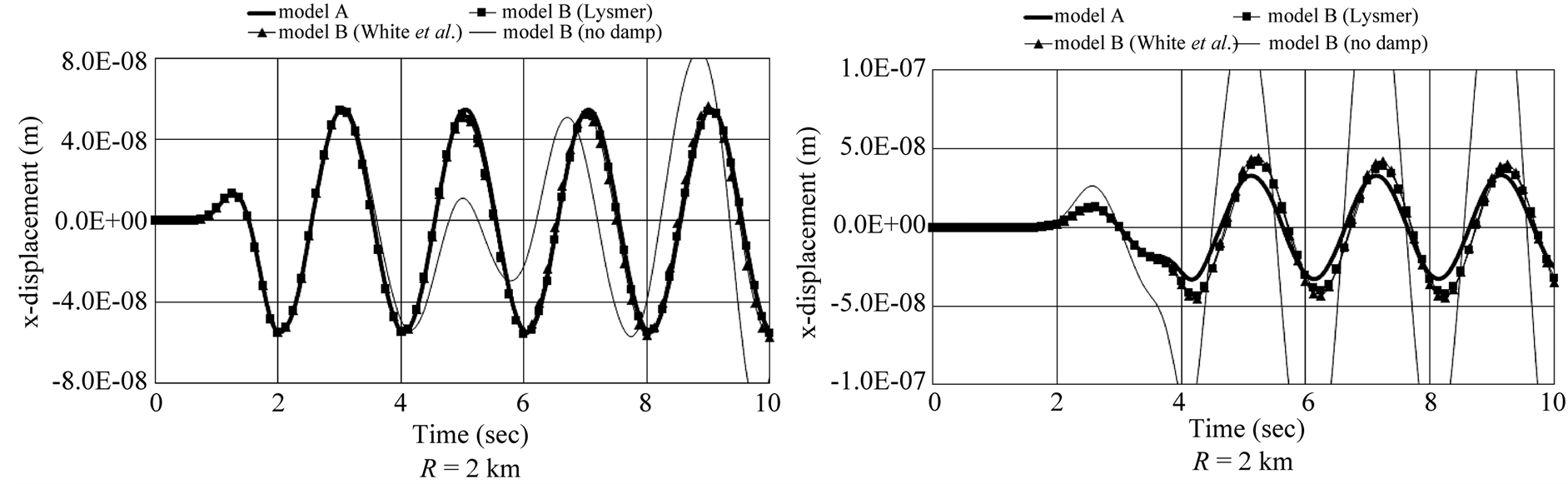
Figure 10. Displacement in x-direction at free surface receiver for rectangular boundary model of Figure 8(b).
Table 3. Absorption ratio of absorbing boundaries wrt position of receiver in Figure 8(a).
Table 4. Absorption ratio of absorbing boundaries wrt position of receiver in Figure 8(b).
In Table 3 and Table 4, the absorption ratios at internal points appear to be larger than those at the boundaries. This is due to the fact that the reflected wave that has been absorbed once is measured at the internal points, which reduces the effect of the reflected wave compared to the points at the boundaries.
For R = 5 km in Table 3, the absorption ratio at the free surface (q = 90˚) is smaller than those of the other points. This can be explained by the elliptic particle motion at the free surface, which makes the wave attack the absorbing boundary with an inclined incident angle due to the surface wave propagating along the surface. Moreover, the absorption ratio reaches approximately 80% in the case with q = 30˚ and the position R = 5 km for the receiver in Table 3 whereas the absorption ratio is approximately 50% in the case with q = 45˚ and R = 5 km in Table4 This result is caused by the arrangement of the dashpots in Model B of Figure 8(a) and Figure 8(b). In Figure 8(a), all the dashpots are installed perpendicularly to the waves propagating radially from the loaded point while the dashpots in Figure 8(b) are installed with an inclination to the wave propagation direction.
This result shows that the performance of the absorbing boundary for waves perpendicular to the boundary is better than that of the absorbing boundary for waves impacting the boundary with an inclination.
5. Conclusion
The performance of absorbing boundaries using dashpot has been examined analytically and numerically. The analytic evaluation was conducted by introducing directly the wave equation for periodic loading into the absorbing boundary conditions. The numerical evaluation was performed by measuring the displacement in numerical models using dashpots. The analytical investigation revealed that the absorbing boundary developed perfectly their performance when the wave attacked the boundary perpendicularly. Moreover, the values of the left-hand side and right-hand side terms in the absorbing boundary equations of Lysmer-Kuhlemeyer were seen to coincide after about one wavelength, which indicated the perfect performance developed for the wave equations generated by periodic loading. Besides, the boundary of White et al. showed defective performance against the S wave. The numerical investigation computed the absorption ratio. The absorption ratio at the free surface appeared to be relatively smaller due to the elliptic particle motion of the surface wave. The absorption ratio indicated comparatively lesser performance of the absorbing boundary for waves impacting the boundary with an inclination than for the wave perpendicular to the boundary. But, besides the boundaries, the absorbing boundaries using dashpots show the superior performance at internal points. A study on the performance of the absorbing boundaries using dashpots is very useful since dashpot boundaries are widely used in finite element analysis. Accordingly, further studies shall be implemented on the absorbing boundaries with inclined angle of incidence including the surface wave for more effective use of the absorbing boundaries.