Keywords
Urban Growth Boundary, Centralization and Suburbanization, Computable General Equilibrium

1. Introduction
Intuitively, increasing the available land, which is an economic resource, should improve social welfare. However, urban planners often implement an urban growth boundary (UGB) policy, which creates compact and densely populated urban forms. Although such policies aim to control the total amount of developable suburban land, it leads to distortion in land markets. Nevertheless, they are frequently defended because they limit urban sprawl and promote the intensive use of public transportation, thereby reducing gasoline use.
Actually, traditional urban economic models show that a UGB policy improves social welfare because it reduces the negative externalities imposed by congestion on the city and directly controls geographical urban sprawl (Brueckner, 2000 [1] ). Since the late 1970s, urban economists have ranked the UGB (with different zones for different land uses, including roads) as the second-best policy after congestion tolling. Originally proposed by Solow (1972) [2] , this view has also found support in several pioneering studies based on monocentric city models (Kanemoto, 1977 [3] ; Arnott, 1979 [4] ; Pines and Sadka, 1985 [5] ). More recently, Bento et al. (2006) [6] showed that, from an efficiency point of view, the UGB and development taxes are the most effective antisprawl policies. However, arguments also exist that the UGB policy is not always powerful. Brueckner (2007) [7] , for example, showed that the welfare gains of the UGB in a monocentric city are small compared with a congestion toll policy.
The UGB’s effectiveness is unclear in a non-monocentric city. The policy may be ineffective because the population can be forced to relocate to more congested areas. Therefore, it may instead be optimal to relocate jobs and populations to less congested areas such as the suburbs, as explained in Anas and Rhee (2007) [8] . However, if more workers reside and work in the suburbs at the optimum compared to a laissez-faire regime, the UGB cannot be the second-best policy. For instance, using a linear polycentric city model that allows for cross-commuting and reverse commuting and in which jobs can be located anywhere, Anas and Rhee (2006) [9] and Ng (2007) [10] showed that the UGB has harmful effects. If open space (or greenbelt) preference is considered, however, the UGB can improve welfare.
Is it likely that the roads in an urban area regulated by a restrictive UGB would be less congested? Assuming that switching from auto to other trip modes is minimal and that road capacity within an area is not increased, congestion per mile would be expected to rise in the central area. At the same time, however, the policy could indirectly reduce travel distances by bringing trip origins and destinations closer together. Thus, what would happen to average congestion levels is unclear. Indeed, a city without restrictive UGB policies may spread out, relatively, and jobs and residences may cluster, resulting in shorter travel distances and less congestion.
While some cities implement a UGB policy, others increase the available land by relaxation of existing UGB or by developing forest and mountain areas or filling water bodies and water-logged areas. In this paper, both restrictive and expansive UGB regimes are examined. A restrictive UGB regulates the development of vacant land in outer suburban zones. With a reduction in the land available for development in these zones, the urban form is expected to become more centralized―that is, the same population will be squeezed into a smaller overall urban land area.
This paper examines the effectiveness and impact of the UGB through a simulation analysis. The remainder is organized as follows. Section 2 describes the model. Section 3 presents the restrictive and expansive UGB policies implemented in outer suburban zones. Section 4 concludes the study.
2. The Model
The simulation model used in this paper is an extension of RELU-TRAN, a computable general equilibrium (CGE) model of an urban economy developed by Anas and Liu (2007) [11] . They present the model in detail and the model explanation in this paper is limited to the overview. The model is applied to the Chicago area. The modeled Chicago area consists of a system of 14 zones in regional economy and land use sub-model (RELU). Zones are connected by aggregation of major and local road and other modes networks in transportation submodel (TRAN) (Figure 1 and Figure 2). RELU and TRAN are sequentially and simultaneously connected. For convenience, the zones are grouped into four rings. Ring 1 is the central business district (CBD), zone 3. Ring 2 is consists of the rest of the city of Chicago, zones 1, 2, 4 and 5. Ring 3 includes all the inner-ring suburbs encircling the city, zones 6 - 10. Ring 4 includes the outer suburbs, zones 11 - 14. Table 1 lists the calibrated land use distribution among these rings in the baseline. Table 2 provides the commuting pattern, namely, the distribution of employed residents in 2000 by home location (origin), job location (destination), and commute mode. Each zone has a housing market, labor market, and output markets for industries. These markets are competitive. The price taking decision makers are consumers, producers, and real estate developers.
2.1. Consumers
There are four different income levels of consumers. In RELU their decision choices are expressed as combinations of 14 residential zones, 14 job zones, 2 housing types (singleand multiple-family housing), and 5 car types by the modeled technological fuel intensity (TFI). Conditional on each discrete bundle, consumers solve the utility maximization problem of the amount of retailed goods and the housing floor space. The budget con-

Figure 2. Modeled network of major roads.
straint is the money income of the consumer, who is paid an hourly wage per workday after travel time for commuting and shopping. However, the consumer can choose not to work and spend non-wage income. The consumers expense on retail goods, housing space, commuting and annual costs of car ownership. Retail prices are effective prices: mill price at the retail location plus the monetary cost of travel from home to the retail location.
RELU is connected to TRAN by the number of trips: the sum of work trips, derived from the residenceworkplace location choice, and non-work trips, derived from the quantity of consumption goods. TRAN is con

Table 1. Calibrated distribution of land (year 2000 baseline).
Table 2. Calibrated distribution of work trips per day (year 2000 baseline).
nected to RELU by travel time and monetary travel cost. In TRAN, consumers, as travelers, decide how to travel from the origin zone to the destination zone: by which mode (auto, public transportation, or other) and which route for auto travelers. Travelers consider the travel cost for their mode and route choices. Congestion imposes a negative externality on travel time.
Although the travel time on the same road is identical for all travelers on that road, evaluation of travel time differs by income group. The monetary cost on the same route also differs by TFI car type, while gasoline consumption differs by driving speed, which depends on congestion. Thus, congestion imposes an externality on gasoline consumption as well. Figure 3 shows the U-shaped relationship between gasoline consumption and driving speed by TFI.
2.2. Developers
Risk-neutral developers are based on a perfect foresight model of building conversions with idiosyncratic cost uncertainty (Anas and Arnott, 1993 [12] ). They construct and demolish buildings, may rent out their building floor space, or buy and sell real estate. Asset prices for vacant land and for each building type are determined so that the expected discounted economic profit, including net rental income, is zero. It is assumed there are six predetermined building types; vacant land, single-family housing, multiple-family housing, commercial, industrial, and non-available land under UGB.
Since the restrictive UGB prohibits the development of vacant land, there are two different effects on land asset values. On the one hand, the building floors and vacant lands inside the UGB, which can continue to be developed or redeveloped, gain in value. On the other hand, the land outside the UGB permanently loses value, because the option to develop that land in the future has become worthless with the UGB. Summing up these two effects, the total value could decrease or increase from the UGB.
Land outside the UGB is potentially developable but not available. Under the expansive UGB, those lands become both available and developable. Before the policy, such land should have had a lower value than the available vacant land and a higher value than the non-developable land. In the benchmark setting, those land values are assumed to be average values of both non-developable and developable vacant land.
2.3. Producers
Profit maximizing industries can produce in any zone and import their inputs from all other zones. The economy includes four industries (agriculture, manufacturing, business services and retail trade). The first three industries produce various goods and services either for selling as intermediate inputs to other industries producing in the region or for export. Retail industry obtains intermediate inputs from the first three industries, but it sells its output only to consumers in the region or exports part of its output.
2.4. Model Structure: General Equilibrium
The equilibrium conditions are pieced together from the demands of consumers, the trips of consumers, the output supply and input demands of firms, and the floor spaces supplied by developers. The relevant markets are the labor market for each labor skill level in each zone (56 equations: 14 zones by 4 skill levels), the residential rental market for singleand multiple-family floor space (28 equations: 14 by 2), the business rental market for commercial and industrial floor space (28 equations: 14 by 2), and the goods market for each industry (56 equations: 4 industries by 14 zones). Solving these equations gives the rental price (per square foot) of each type of floor space, the hourly wage for each skill level, and the output price for each industry in each zone.
2.5. Measuring Welfare
The aggregate welfare gain is measured by the summation of the compensative variations (CVs) and the gain or loss from real estate. CVs are the differences between the utilities before and after the policy as evaluated by consumers, calculated by income group and job status. The gain or loss from real estate is the change in aggregate real estate values by the policy. Both absentee and non-absentee landlords own real estate in the city, but the former reside outside the city and the latter inside. The gain or loss from real estate is treated as the welfare of non-absentee landlords. Absentee landlords’ real estate gain or loss is a drain from the city. Tenured residents represent approximately 60% - 70% of the total. Although the model allows for both housing and non-housing buildings, it is assumed that non-absentee landlords account for a higher proportion than tenured residents. In the benchmark setting, 90% of landlords are non-absentee landlords and 10% are absentee landlords. For the purpose of comparison, the Pigouvian congestion toll policy is simulated. In this case, welfare is evaluated as the summation of the CVs, the gain or loss from real estate, and the toll revenue.
3. Impacts of UGB Policies
In this section, the restrictive and expansive UGB policies are examined. The restrictive UGB applies at every 5% reduction in the base of the undeveloped vacant land available in the outer suburban rings. Likewise, the expansive UGB will increase the base of the developable vacant lands in the outer suburban rings. In the model, buildings are both constructed on vacant land and demolished to create vacant land. At the equilibrium, the floor space of buildings constructed is equal to that of buildings demolished in each zone. Thus, the UGB violates the equilibrium condition by changing developable vacant land in the outer suburban zones, and the economy moves to a new equilibrium. This is the first impact of the UGB.
The restrictive UGB of entire available undeveloped land in the zone does not mean that no development occurs. In fact, two types of development can still take place. One is “infill development”, which means that vacant land areas within the city can (and are more likely to) be developed, since outer suburban vacant land is unavailable. The second type is “redevelopment”, which means that as the urban area adjusts to a new general equilibrium (in response to the UGB), buildings within the UGB can be demolished and new ones constructed instead.
3.1. Stock
Figure 4 shows the different effects of the restrictive and expansive UGB policies on each building type in the different rings. Since the restrictive UGB pushes economic activities such as jobs, residents and shopping customers toward the city center, vacant land decreases not only in the outer suburban rings but in all the rings. Moreover, it reduces faster in the outer suburban rings than it does in the inner rings. However, outer suburban vacant land does not reduce as much as it would under the restrictive UGB. For example, when the restrictive UGB index is −1 (i.e., 100% of the originally vacant land in the base case is unavailable for new development), the available vacant land decreases by approximately 60%. This drop occurs because, as job and residence location demands shift to the inner rings for the UGB policy, some existing buildings are demolished. The vacant land in the other inner rings decreases by infill and redevelopment, as economic activities move from the outer suburbs.
These figures show that each type of building stock in the outer suburbs decreases while most types of building stock in the other inner rings increase. The exceptions to this are that single-family housing stocks in the CBD and city decrease to make room for higher-density apartments and commercial buildings. Infill development, therefore, is a direct consequence of a restrictive UGB. Changes in stock are in the direction of higher structural density, since the stock of low-density structures such as single-family housing reduces while that of higher-density apartments or other building stocks increases.
In the expansive UGB case, the effects on stocks are in the opposite direction. Since more land is developable, developers construct more buildings. This provides more lower-rent floor supply to the market and causes “outfill” development; in other words, buildings in the inner rings are demolished, while single-family housing increases owing to construction and redevelopment.
3.2. Mode Choice, Travel Time, and Gasoline Consumption
Figure 5 shows the changing pattern in the number of trips by each mode. As the UGB becomes tighter, auto-

Figure 5. UGB-induced changes in number of trips by mode.
trips decrease, while public transportation travel and other trips increase. Considering with the location choices, this occurs because the most frequently used mode in outer suburban trips is the auto. When consumers move from an outer suburban rings to inner rings, many of them change their travel mode from auto to other modes, because the roads near the CBD are heavily congested, and an efficient public transportation system is available. Hence, even though the number of auto commuters increases in the inner rings and decreases in the outer suburbs, auto commuting decreases as a whole. In this sense, the restrictive UGB achieves one of its purposes, namely, an increase in public transportation ridership. However, the number of trips decreases over all. This reduction is mostly explained by the decrease in the number of non-work trips, because of the congested roads and costly travel cost near city center.
Figure 6 shows the percentage change in average travel time by each mode under the UGB. Travel time per trip for all modes decreases as the UGB becomes tighter. Travel time for public transportation and the other modes decreases because the travel distance per trip is lower. Travel time for auto commuters is affected by the decrease in travel distance and the congestion levels. Because the UGB pushes economic activities toward the city center, trips increase near the center and decrease in suburban zones, and thus, driving speed decreases in the center and increases in the suburbs. Under the expansive UGB, travel distances therefore increase, while congestion decreases in the center and increases in the suburbs.
Figure 7 shows the impact of the UGB on gasoline consumption and its two main components, vehicle miles of travel (VMT) and gallons per mile (GPM). As the UGB becomes tighter, gasoline consumption decreases. Most of this decrease is explained by a reduction in VMT, although the reduction in gasoline consumption is less

Figure 7. Gasoline consumption, vehicle miles of travel (VMT) and gallons per mile (GPM).
than that in VMT because the GPM increases from two contrary forces. On the one hand, the amount of driving on congested city roads increases, and driving speeds decrease. On the other hand, suburban non-congested roads become even less congested and driving becomes smoother. The first effect increases GPM, but the second might or might not decrease it, since too high driving speeds require greater gasoline consumption.
3.3. Welfare
3.3.1. UGB Impact on Welfare
The most direct impact on the urban economy from the restrictive UGB is the removal of available land resources from the market, which negatively influences the economy. Even so, it is possible that the UGB improves welfare by reducing the negative effects of congestion. In the Table 3, the Regime 1 (Benchmark) shows the impacts of 10% restrictive UGB and 10% expansive UGB on urban economy. Opt. expresses the optimal level UGB. Because consumers move to locations that offer convenient public transportation and VMT decreases 0.09%, the 10% restrictive UGB reduces the effect of congestion. However, such locations are close to the center, where roads are congested. As a result, the number of auto trips increases on congested roads and decreases on less congested roads, while more trips are made by public transport.
The UGB also has rent and wage effects, mediated through the general equilibrium. Since the restrictive UGB regulates the development of vacant land, the available land becomes scarcer, and floor rent increases. The change in rent is 1.78% in the outer suburbs where the UGB is implemented. This is much faster than it is in the other rings. Since rent increases, producers substitute other inputs for floor space and labor demand increases. As economic activity shifts toward the center, the gross product in the outer suburban rings decreases. However, the wage increases from 0.01% to 0.1% since labor demand increases. While labor supply decreases in the outer rings, it increases in the other inner rings.
Although higher wages and lower travel time benefit employed consumers, the other negative effects, primarily higher rents, are more powerful. Thus the general equilibrium effect decreases consumer utility. An increment in the per unit land value within the UGB because for reduced land supply is a possible positive effect. Thus, annualized total land value increases $11.2 per person. It is also possible, theoretically, that total land value decreases with reduced land supply under a restrictive UGB. In an expansive UGB, however, many of the above effects work in the opposite direction. For example, the expansive UGB adds available land to the market in outer suburban zones and rents decrease 1.67%. Location choices are therefore suburbanized and VMT increases 0.1%. Congestion near the city center decreases, while traffic moves out to the suburbs. At the same time, the number of public transportation trips decreases 0.14%.
3.3.2. Absentee Landlords
In the benchmark setting, it is assumed that 10% of landlords are absent from the city. With more absentee landlords, the gain or loss from the real estate market will drain from the city and vice versa. Figure 8 shows social welfare levels with 0% and 20% absentee landlords, respectively. The restrictive UGB increases the total building value in the city. With more absentee landlords, the impact of a restrictive UGB is greater and causes more welfare loss because relatively high gains from real estate values flow from the city. In the case of an expansive UGB, however, asset values in the city fall. Therefore, citizens suffer a smaller proportion of the real estate losses, and welfare gains increase.
3.3.3. Higher Evaluation of Vacant Land Value outside the UGB
An important variation in the literature treats the UGB policy in a context in which consumers have a positive preference for additional open spaces created by the UGB. If open spaces positively affect the economy, vacant land outside the UGB should be evaluated higher than in the benchmark settings. Central Park in New York City is a good example of the UGB as a welfare-improving policy. Anas and Rhee (2006) [9] , Bento et al. (2006) [6] , and Ng (2007) [10] modeled a UGB that incorporated a preference for open spaces. Bento et al. (2006) [6] showed that the UGB, coupled with a property tax, is a welfare-improving policy if consumers prefer open spaces created by the UGB. Similarly, Anas and Rhee (2006) [9] and Ng (2007) [10] showed a welfare loss from the UGB if consumers do not value open spaces.
Figure 9 shows the social welfare level under the restrictive UGB when open spaces are evaluated higher than in the benchmark simulation. In the benchmark settings, the average value of non-developable vacant land
Table 3. UGB under different regimes.
Continued
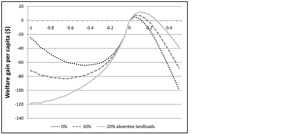
Figure 8. Welfare levels based on the percentage of absentee landlord-owned real estate.

Figure 9. Welfare levels with an evaluation of open spaces.
outside the restrictive UGB is 20.2% of the average value of developable vacant land at the base. The high value, the medium high value, the medium value of the land outside the restrictive UGB are set as 32.6%, 29.6%, and 27.6%, respectively. Then the maximum social welfare gains are $23.44, $9.42, and $2.66 at the optimum restrictive UGB levels, 55%, 40%, and 35%. As the UGB becomes tighter, social welfare gains decrease, hitting $0 at UGB levels of 100%, 75%, and 50%, respectively.
3.4. Comparative Statics
3.4.1. Comparing Different Elasticity
How would the results differ if the market reacted to the UGB more elastically? A comparison of UGB results across the four regimes is presented in Table 3. Regime 1 is the benchmark setting. In regimes 2 - 4, the elasticities are raised by increasing the dispersion parameters by 50% for the construction and demolition probabilities of developers (regime 2), the mode choice probability of consumers (regime 3), and the consumer choice probability in locations-housing type-car type in RELU (regime 4). To keep the same base, these probabilities are recalibrated. In each case, a 10% restrictive and a 10% expansive UGB are assumed for comparison purposes, besides the optimal UGB. Most of the discussion for 10% restrictive UGB applies conversely to the 10% expansive UGB.
In regime 2, the economy adjusts to the impact of the UGB by constructing and demolishing buildings. The results show that more buildings are constructed. The impact of the more elastic mode choice in regime 3 is small. A comparison of impacts between regimes 3 and 4 (more elastic RELU probability) suggests that the increase in transit trips is greater in the latter. This is because, in regime 4, jobs and residents move from the outer suburban rings to the inner rings. Since public transportation and the other modes in the inner rings are more convenient than in the outer suburban rings, trips by these modes increase. This increment is more than the increase in regime 3. Hence, a reduction in gasoline consumption and VMT is a direct result of the UGB. Gasoline consumption decreases most in regime 4, followed by regimes 1, 3 and 2. This order is consistent with centralized location choices.
Figure 10 shows how the UGB affects social welfare under different regimes. Regimes 1, 3 and 4 have similar welfare levels, but regime 2 shows a relatively large change in welfare. Because the UGB affects the land market first, it is reasonable that regime 2, in which the elasticity of the construction and demolition probabilities is higher, shows a relatively large impact on welfare compared to the other regimes. In all regimes, however, welfare improvement peaks at 10% - 25% in the expansive UGB, although the impact is moderate. Under the restrictive UGB, welfare keeps decreasing in regime 2. In regimes 1, 3 and 4, as the restrictive UGB becomes tighter, social welfare decreases at the beginning, and then increases to some extent. Since the floor supply is less flexible, the real estate value increases relatively more. Thus the gain from real estate value exceeds the loss in CV under this UGB.
3.4.2. Comparing the Effects of Pigouvian Congestion Tolling and the UGB
Economists know that externalities are best internalized by imposing the Pigouvian congestion tax in the margins across which externalities exist. In this subsection, the welfare gain in the Pigouvian congestion toll is compared with that of the UGB of regime 1, benchmark setting. The Pigouvian toll internalizes both time delay and gasoline consumption externalities on all roads. With a congestion toll, social welfare is the summation of the CV, the gain from real estate, and the toll revenue. Table 3 shows that welfare improvement under the Pigouvian toll is valued at $503. Since the welfare improvement under the optimal UGB is equal to $12.83, the

Figure 10. Welfare levels under different UGB regimes.
UGB achieves only 2.5% of the welfare improvement generated by the Pigouvian toll. This modest improvement relative to the congestion toll policy is consistent with the results presented by Brueckner (2007) [7] , where the UGB achieved only 0.7% of the welfare improvement derived from the toll, although our optimal UGB is expansive. Social welfare can be roughly divided into a negative CV, positive real estate value gains, and toll revenue under the Pigouvian toll. Under the optimal expansive UGB, these are a positive CV and a negative real estate value gains.
Table 3 shows some of the other impacts of the Pigouvian toll and the UGB. The first impact of the toll is an increase in the monetary travel cost for auto travelers. Consumers switch to the other two modes when it is convenient to do so or move to locations nearer to the center. As a result, gasoline consumption, VMT, and GPM decrease, and travel time becomes shorter. Thus, in addition to altering the degree of change, the optimal UGB and congestion toll affect the economic variables in opposite ways.
4. Conclusions
Although congestion in a city gives rise to negative externalities, it is reasonable to expect that a restrictive UGB reduces the negative effect of congestion for three main reasons. First, the city becomes more compact, and therefore, travel distances decrease. Second, residential and job locations become centralized, meaning that trips by public transportation or other modes are more convenient. Third, residential properties appreciate in the real estate market. However, the most direct impact of a restrictive UGB is the removal of developable vacant land, which is an economic resource, from the market. Thus, the UGB has both positive and negative effects.
In this paper, both restrictive and expansive UGB regimes were examined in a polycentric city. The presented simulation results based on the Chicago metropolitan statistical area showed that an expansive UGB positively affects social welfare. It was also shown that a restrictive UGB improves social welfare if the vacant land outside the UGB is evaluated as an open space. Even if the restrictive UGB does not always improve social welfare, it succeeds in achieving other objectives, such as reducing gasoline consumption and increasing use of public transportation. The proportion of absentee landlords is also an important determinant of welfare gains, since the gain or loss from a UGB policy in the real estate market is drains from the urban economy.
Acknowledgements
I would like to thank Professor Alex Anas and Professor Richard Arnott for their insightful comments and advices.
Appendix: Data and Calibration
Deciding on the model’s parameters was a mixture of fixing some at reasonable values and calibrating others such that the elasticity relationships concerning location demand, housing demand and supply, and the labor market were within the ranges of estimates in the literature. In this appendix, the datasets used for calibration is explained first. Then the calibrated model fit to the data is explained.
Data
A variety of datasets were utilized to calibrate RELU-TRAN. Travel times and work trips from residences (origins) to workplaces (destinations) by income and mode of travel (car, mass transit, and non-motorized) came from the 2000 Census Transportation Planning Package. From this same source, jobs by zone of workplace and estimates of wages by place of work were also determined. Non-work trip frequencies from residence locations (trip origins) were estimated from the Home Interview Survey for the Chicago metropolitan statistical area (MSA).
Residential housing stock was derived from the 2000 Census and non-residential building stock and floor space prices from COSTAR data. Residential housing prices and rents for floor space in singleand multiplefamily housing were inferred from an imputation procedure that used Public Use Micro Sample data. Land use files of the Northeastern Illinois Planning Commission were used for the vacant developable land and land use by building type in each model zone; from these, the structural density of buildings by type was constructed as a zone-average floor area per acre. The industries and inter-industry trade-flow relationships were obtained by following IMPLAN’s economic modeling system, as were the expenditure shares by intermediate input categories. Car costs were from the American Automobile Association (AAA, 2005) [13] and the Bureau of Labor Statistics.
The Model’s Fit to the Data
Since the model is an extension of RELU-TRAN that includes a choice among five car types that differ by TFI (Figure 3) and precise calculations of gasoline use, VMT, MPG, and speed, it required a calibration adjustment that drew on additional data. Data targets were constructed to be matched as closely as possible by the calibration. Regional Transportation Assets Management System (RTAMS, 2000) [14] data, which contains an aggregated version of 2000 census transportation planning package data for the Chicago MSA, were used to target the number of jobs and residents by zone, work trip patterns by mode of commuting, and average travel speed. VMT, gas use, and MPG targets came from Illinois Travel Statistics (IDOT, 2000) [15] . The targeted car distribution by TFI was constructed from NHTS (2001) [16] .
Table 4 shows how the calibrated model fit the targets.
Table 4. Fit of the calibrated model to the targets constructed from data.