Could Sequential Residual Centering Resolve Low Sensitivity in Moderated Regression? Simulations and Cancer Symptom Clusters ()
1. Introduction
Low sensitivity in quadratic and moderated multiple regression (QMMR) analysis has challenged researchers ever since computer software to conduct regression became available in the 1960s. A major cause is multicollinearity, or shared variation among predictors that inflates standard errors of regression coefficients. Progress in overcoming this predicament suffered a setback several years ago when it was proven that the common practice of mean centering in moderated regression cannot alleviate multicollinearity among variables comprising an interaction, but merely masks it. Residual centering (orthogonalizing) is unacceptable because it biases coefficients for predictors from which the interaction(s) derives, despite the non-biased coefficient for the highest-order polynomial interaction, thus precluding interpretation of moderator effects [1,2].
In this article, I propose, derive, and validate the application of residual centering in sequential re-estimations of a moderated regression—sequential residual centering (SRC)—in order to obtain unbiased conditioning of multicollinearity across the highest-order interacttion and related terms. Across simulations (n = 250 and 1000), SRC reduces variance inflation factors (VIF) regardless whether all random variables are normal, nonnormal, or have similaror different-shaped non-normal distributions, and regardless of the pattern of regression coefficients across the set of predictors. For any predictor, the reduced VIF is used to derive a lower standard error of its regression slope parameter.
A sample of cancer symptoms (n = 268) illustrates SRC, which allows unbiased interpretations (direct and post hoc) of symptom clusters. SRC facilitates unbiased interpretations of 1) the nature (magnifier and/or buffering) of moderator effects; and 2) total net moderator effects from an interaction term and its related lower-order polynomial terms using the standardized regression. In addition, the simulation and cancer sample demonstrate extensions to SRC that lower standard errors even further by conditioning predictors to be uncorrelated with quadratic terms or control/secondary variables—predictors from which the interaction term(s) are not strictly derivative. SRC can be applied efficiently to alleviate multicollinearity after data collection and allows unbiased detection and interpretation of moderator effects. This innovation could advance synergistic frontiers of research and evaluation in biomarker and symptom cluster investigations, other areas of medicine, and more broadly, across the sciences and social sciences.
2. Background
When original scores of uncentered variables are used in QMMR, estimates of slope coefficients for the one-way predictors of simple effects may appear inflated to the extent that these terms are correlated with higher-order predictors. Indeed, when these one-way predictors are normally distributed, mean centering (i.e., subtracting the mean value from each score) typically yields lower values for parameter estimates of simple effects. For many years, mean centering was recommended to alleviate multicollinearity from the use of arbitrary ordinal measurement scales—referred to as “inessential ill-conditioning”—in order to prevent biased and inflated parameter estimates, as long as the one-way terms that serve as components of higher-order terms are normally distributed [3-5].
However, in the past decade, Echambadi and Hess [2] proved that mean centering cannot alleviate multicollinearity in QMMR; the procedure merely masks the presence of underlying multicollinearity, although as they point out, more than twenty-five years ago Belsley [6] revealed that mean centering is ineffective in alleviating multicollinearity in additive models. Deflated parameter estimates for simple effects occur because mean centering changes the actual specified model that is tested— parameter estimates shift from controlling remaining predictors when they are at the value of zero to when they are at their mean values.
Common multicollinearity diagnostic tools such as bivariate correlations and variance inflation factor (VIF) values assess each predictor separately (and not the global set of predictors simultaneously). Therefore, when used alone, each tool cannot be taken to be fully sensitive to detect problematic multicollinearity in different contexts [7]. Specificity is not an issue, however, since high VIF values always reveal situations of high multicollinearity, even as other situations of high multicollinearity can occur without inflated VIF values [8]. When oneway predictors are normally distributed, mean-centered data usually mask the full extent of multicollinearity [6]. Therefore, the use of multiple diagnostic tools is recommended to assess multicollinearity in uncentered—and not mean-centered—data when one-way predictors are normally distributed, although this practice does not usually resolve the serious dilemma about how to remedy problematic multicollinearity after the data have been collected [2].
2.1. Residual Centering (Orthogonalization)
In contrast to mean centering, residual centering (i.e., orthogonalization) does alleviate multicollinearity, although as we shall see, only partially and by biasing estimates of the slopes of lower-order predictors. Furthermore, residual centering alleviates multicollinearity that stems from normal, non-normal, or asymmetric predictor distributions. Therefore, the quadratic or interaction term is fully independent from the one-way terms on which they are based [9].
Lance [9] advanced the original procedure to estimate a QMMR by residually centering—orthogonalizing—the highest-order term(s). Here I specify a third-order polynomial regression testing the three-way interaction (wxz):
 (1)
(1)
where b0 is the intercept and e is the residual.
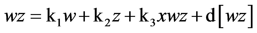
Then regression without a constant term is used to partial all oneand two-way terms from the three-way term, xwz:
 (2)
(2)
where d[xwz] is the residual. Equation (2) can be re-expressed as:
 (3)
(3)
Substituting d[xwz] for xwz in Equation (1), I re-estimate this raw regression as a residual centered regression, factoring out the variance in xwz that is shared with oneand two-way predictors:
 (4)
(4)
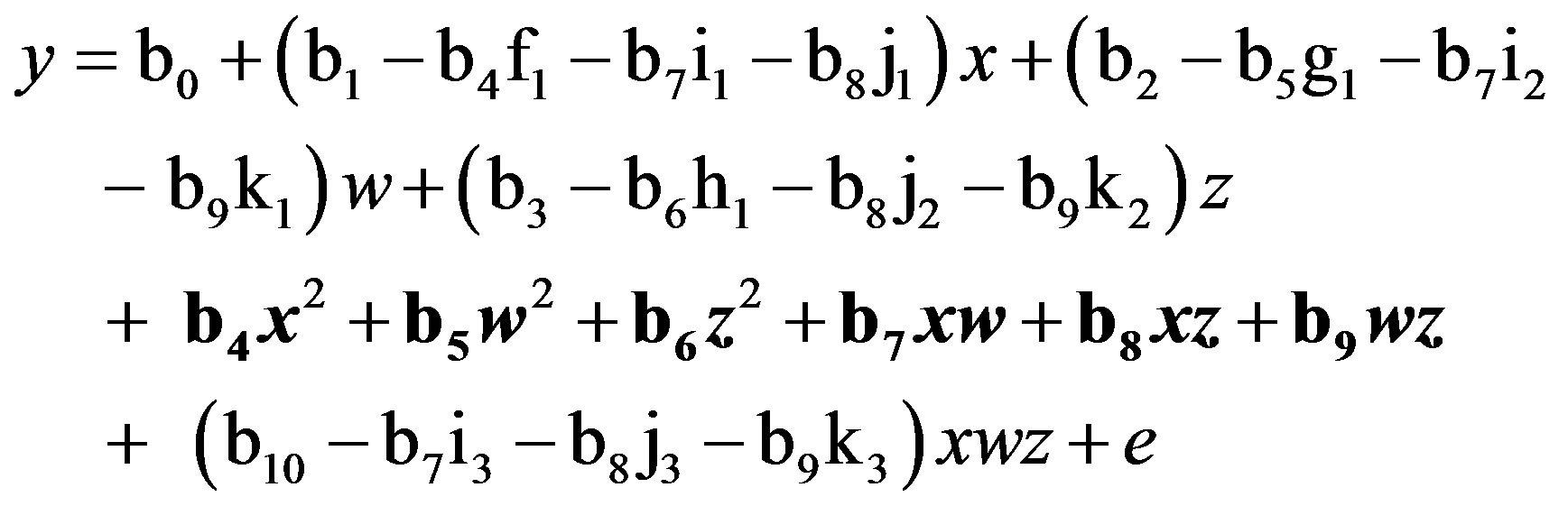
Finally, substituting Equation (3) into Equation (4), this residual centered regression is equivalent to:
 (5)
(5)
Thus, the term in bold, b10xwz, is unchanged (i.e., nonbiased). Its standard error does not change either, as I show later, although its variance inflation factor (VIF) falls because inessential multicollinearity is alleviated. In contrast, the changes in all oneand two-way terms (such as the one-way simple effects in a QMMR testing a twoway interaction) represent systematic biases [1], which Lance [9] did not recognize in recommending the procedure. Instead, he attributed the changes in parameters of lower-order polynomial terms to improved estimation from reduced multicollinearity [2,9].
2.2. Biased Interpretations from Residual Centering
In residual centering, only parameters for the highestorder polynomial term(s) are unbiased—lower-order polynomial terms (simple effects and any quadratic terms and interactions) now become biased. This situation precludes post hoc assessment of the nature and strength of quadratic and moderator effects across the range of x since unbiased estimates for all of these terms are necessary in different approaches [3,5,10-13]. Similarly, direct interpretations (without these post hoc assessments) in residual centering are also biased.
A common procedure provides a basis for comparing two types of direct interpretations. In the case of the simplest moderated regression equation specifying only a two-way interaction, some researchers directly interpret the degree to which the residually centered interaction term moderates the primary x-y relationship, based on the signed coefficient rule—a comparison of the signs of the coefficients for the x term and the interaction term ([9]; for applications, see [14-17]). For instance, a decreasing primary x-y relationship that is lowered further reveals a magnifier effect, but if the primary relationship were increasing, lowering it would instead represent a buffering effect. This direct interpretation is possible because the residually centered two-way interaction term is fully independent of the one-way terms from which it derives [9]. The rule may be used in unstandardized or standardized regression. Unfortunately, the signed coefficient rule is not always reliable to yield correct interpretations of the moderator effect, depending on the coding scheme for the moderator variable. This dilemma occurs when different participant subgroups revealed by the interaction term are correlated with the y variable but in the opposite direction, as Aguinis [18] demonstrated using a binary moderator variable coded as 0 and 1.
The direct interpretation using the signed coefficient rule reveals the unique net moderator effect contributed by the interaction term, which should not be confused with the total net moderator effect, a summation of standardized predictors based on the interaction term and all lower-order polynomial terms (interactions and one-way terms). Indeed, as the current study will show, it is possible for the unique and total net moderator effects to have different signs—a situation which could signal a similar type of unreliability in the signed coefficient rule for interpreting the unique net moderator effect when the lowest score of ordinal moderator variable(s) is coded as 0. In any event, the total net moderator effect, which does not suffer from this dilemma, is based on the interaction term and—except for the x term—all lower-order polynomial terms (interactions and one-way terms). For this type of direct interpretation to be commensurate with post hoc procedures for interpreting moderator effects, which necessarily involve the highest-order interaction term and all lower-order polynomial terms (interactions and one-way terms), the sign of the standardized coefficient for the x term needs to be compared to the sign of the total net moderator effect, which is the sign from the sum of the standardized coefficients for the interaction and all derivative terms (except x). This reliable adaptation to the signed coefficient rule will be used in the current study, which will validate an innovative approach to residual centering that avoids bias.
Standardized predictors may facilitate direct interprettation. Lance [9] illustrates a two-way interaction model in which the one-way predictors that serve as components of the two-way interaction are standardized. Lance used these standardizations to create a correlation matrix of predictors with near-zero cross-correlations showing that residual centering results in complete orthogonalization (which is necessarily the case even when these same predictors are unstandardized). Thus, a product or powered term and its zero-order component terms are fully independent and yield separate, non-overlapping estimates for interaction, quadratic, and main effects. (Standardization, it should be noted, transforms one-way variables to become mean-centered, such that simple effects become main effects.) Standardization allows predictors to be compared to identify those with stronger effects1, although when non-arbitrary scaling metrics are used, only unstandardized estimates should be conducted, as Lance [9] recommends.
Unfortunately, advantages afforded by standardization are insufficient—despite orthogonalization, residual centering introduces systematic bias into the parameter estimate, which may lead to an incorrect direct interpretation. Systematic bias in the x coefficient from a two-way model can change its sign or whether it is statistically significant, prompting wrong conclusions about the nature of the moderator effect. Moreover, distinctions between full moderation (i.e., both x and the interaction term are statistically significant) and partial moderation (i.e., only the interaction term is significant) [20] may be noted incorrectly in twoand three-way models.
3. Methods
Improvements to the method of residual centering will be developed to eliminate various biases, including biases in regression parameters of lower-order polynomial terms, introduced when the original residual centering procedure [9] is applied. The subsequent sections explain the improved procedure as well as the simulations and clinical data to validate and demonstrate it.
3.1. Sequential Residual Centering (SRC)
I developed the sequential application of residual centering, or sequential residual centering (SRC), to remove systematic biases in regression parameters of lower-order polynomial terms during a study of cancer symptom clusters [21]. A QMMR equation with a three-way term is estimated using residual centering, as described earlier. The QMMR is then re-estimated by residually centering only the two-way terms. In a subsequent re-estimation, only the one-way (simple effect) terms are residually centered. In each re-estimation, the residual centered terms partial out not only the lower-order polynomial terms, but also all derivative higher-order polynomial term(s), in order to be consistent with terms that were factored from the original raw regression and any prior re-estimations.
For instance, non-biased estimates of the two-way terms from (1) are derived in residualizing regressions:
 (6)
(6)
 (7)
(7)
 (8)
(8)
 (9)
(9)
 (10)
(10)
 (11)
(11)
Although Equations (9)-(11) residually center the twoway interaction terms, it may not be clear why the threeway interaction term, xwz, is also a predictor in each of these equations. These specifications partial out the inessential multicollinearity this three-way interaction term shares with each two-way interaction term that is being residually centered. Otherwise, inessential multicollinearity within the overall SRC regression (to be derived next) would remain between each residual centered twoway interaction term and this three-way interaction term. Thus, the specification of this three-way interaction in Equations (9)-(11) will result in non-biased regression slopes (b) for all residual centered, two-way interaction terms within the overall SRC regression—which also includes xwz—represented by Equations (12) and (13) below.
As before, Equations (6) through (11) can be re-expressed to derive d[x2], d[w2], d[z2], d[xw], d[xz], and d[wz], which substitute in Equation (1). I re-estimate this raw regression as an SRC regression, factoring out the variance in these two-way terms that are shared with the remaining terms:
 (12)
(12)
Finally, substituting Equations (6) through (11) into (12), this QMMR with residually centered first-order (two-way) terms is equivalent to:
 (13)
(13)
Again, all six two-way terms (in bold) are unchanged (i.e., non-biased). This result is expected because multicollinearity does not bias estimates of regression slope parameters (unless it is extremely high) even as it inflates standard errors [22]. Therefore, SRC is expected to yield b estimates that are identical to those derived from the raw regression in Equation (1). A similar set of derivations results in unchanged (i.e., non-biased) estimates for all three one-way terms (i.e., x, w, z).
If the three-way interaction term was not also specified in Equations (9)-(11), the regression slope parameter estimates in Equations (12) and (13) for the two-way interaction terms—i.e., b7, b8, and b9—would shift as a result of this specification bias. As before, the standard errors for these regression slope parameters also do not change, and their VIF values fall because inessential multicollinearity is alleviated. Towards the end of this section, I will use these reduced VIF values to derive the “essential” portion of each standard error estimate that is not inflated by “inessential” multicollinearity. The lower values of these essential standard errors (ESE) will be used in place of the corresponding inflated standard errors.
SRC conditions out the inessential multicollinearity among the highest-order interaction and each of the successively lower-order polynomial terms—for instance, in Equations (5) and (13). This multicollinearity should be expected and constitutes “inessential ill-conditioning” due to the inclusion of overlapping terms that tap overall effects and derivative subgroup effects. In the absence of SRC—for instance, in the raw regression [Equation (1)]—inessential ill-conditioning results in inflated variance inflation factors (VIF).
The remaining multicollinearity in SRC regressions, such as Equations (5) and (13), occur among predictor terms either of the same polynomial order (e.g., among the two-way terms) or across orders (across the one-, two-, and three-way terms) that do not involve one-way terms for the component variables of the interaction(s) or their derivative higher-order term(s). This multicollinearity constitutes “essential ill-conditioning” due to predictor terms that overlap not as a result of the modeling artifact of including necessarily related terms of different orders, but that overlap across altogether different variables within the same polynomial order, or across orders, of predictor terms. For instance, the quadratic terms (x2, w2, and z2) are not derivative terms of any of the twoor three-way interactions involving x, w, and/or z as components. If control or secondary predictors were specified, multicollinearity related to these terms would also constitute essential ill-conditioning. Thus, this remaining “essential” multicollinearity within the VIF—the VIF from Essential Ill-Conditioning, or Essential VIF (EVIF)—is real and not a modeling artifact. Compared to the VIF, EVIF provides a better and more reliable indication as to whether the remaining essential ill-conditioning constitutes a level of multicollinearity that may undermine the validity of parameter and standard error estimates.
Each one-way term, quadratic term, and interaction term includes variation that is: 1) shared with lowerand higher-order polynomial terms based on the same component variables [inessential ill-conditioning—Equations (2) and (6) through (11), for instance, partial it out]; 2) shared with non-derivative quadratic terms and any remaining predictors that involve different variables [essential ill-conditioning]; and 3) unique only to that term. Since a derivative term, by definition, incorporates shared variation with lower-order terms upon which it is based, and with higher-order terms to which it contributes as a component, this shared portion of overall variance (i.e., inessential ill-conditioning) should not be included in estimating the standard error of the b parameter for this derivative term. Even if an interaction term or other predictor shares most of its variation with its related lowerand/or higher-order terms, the contribution of the unique variation from this term in estimating the standard error of its b parameter should not be distorted by data reflecting its shared variation with related terms.
In the final step, I return to the raw regression to condition away inessential ill-conditioning from each predictor or interaction term—that is, the portion of shared variation with related terms that serves to inflate the standard error. The EVIF values from the series of SRC regressions, including Equations (5) and (13), are applied within the raw regression [Equation (1)] to determine the essential standard error (ESE) for each b parameter—i.e., the estimated standard error in the raw regression which is influenced by essential ill-conditioning but not by inessential ill-conditioning. For any predictor or interaction term (e.g., xw), the variance of the b parameter estimate is related to the VIF as shown by Shieh [23]:
 (14)
(14)
where σ2 is the variance of the regression residual term and  is the sum of the squared mean-centered values for xw. In place of software output for σ2 and
 , the value for c can be calculated directly using the raw regression output for V(bxw) and VIF(xw), as follows: c = V(bxw)/VIF(xw).
Then, replacing VIF(xw) in (14) with the EVIF value for bxw from the SRC regression (13), while retaining the value for c, yields the Essential V(bxw): Essential V(bxw) = c EVIF(xw).
Taking the square root of the Essential V(bxw) yields the Essential Standard Error (ESE) of the bxw parameter. Finally, when testing the statistical significance of bxw, replacing the standard error (SE) from the raw regression with ESE yields a larger z-statistic (in absolute value).
In summary, for each predictor, although the raw regression results in the same standard error obtained by the corresponding SRC regression for the residual-centered specification of that term, the SRC regression yields a lower VIF value, which is equivalent to the EVIF. The EVIF captures the extent of essential ill-conditioning within the standard error of a given b parameter. It permits us to calculate a lower standard error for the corresponding b parameter in the raw regression (i.e., the ESE) based only on the portion of the data constituting the original raw predictor variable that does not contribute to inessential ill-conditioning in the raw regression. Thus, in SRC, the QMMR is re-estimated sequentially to derive valid parameter estimates for each order of terms. Each re-estimation partials away the portion of inessential multicollinearity that would otherwise bias parameter (and standard error) estimates for a given order of terms. Finally, it should be noted that while I illustrated SRC using the three-way specification testing wxz in (1), a specification testing one or more third-order curvilinear interactions, such as wx2, would provide a similar derivation.
3.1.1. SRC with Standardized Scores to Assess Total Net Moderator Effects
The lack of systematic bias in parameter estimates from SRC, in contrast to the original residual centering [9], means that SRC can be used with standardized scores of arbitrarily scaled predictors to assess total net moderator effects across predictors based on the sum of their standardized slope parameters. The independence of these standardized predictors, which permits their sums, is supported when SRC reduces their correlations to low levels. An adaptation of the signed coefficient rule is used to compare the coefficient signs from this sum and the primary predictor to determine the total net moderator effect (net magnifier or net buffering).
A caveat is in order. When conducting an unstandardized raw QMMR, the automatically generated standardized regression output is incorrect because the statistical software does not properly standardize the higher-order terms. As Friedrich [19] clarified, the correct standardized values for a quadratic or interaction term is based on the product of the standardized zero-order (one-way) component variables for that term (and not on the automatic standardization of the higher-order term). The standard errors for these correct standardized values still remain incorrect, however. Therefore, statistical significance should be based on the correct t-statistics for these terms from the unstandardized raw QMMR.
3.1.2. SRC Extensions to Condition for Additional Multicollinearity
The twoand three-way interactions in residualizing regression Equations (6) through (11) are not derivative terms of the set of quadratic predictors in (1) [i.e., x2, w2, and z2]. However, the quadratic and interaction terms are indirectly related to each other since they are based on the same one-way derivative terms [i.e., x, w, and z]. This overlapping variation appears to be an additional—although indirect—source of inessential multicollinearity affecting quadratic and interaction terms despite their non-derivative relationship. If this is correct, using SRC with Quadratic Terms (SRC-Q) to further condition this inessential multicollinearity should provide even lower EVIF estimates than SRC, along with equivalent estimates for the regression slopes and standard errors.
In order to expand SRC into SRC-Q, I will add: 1) the three quadratic terms to each of the residualizing regressions of the four interaction terms; and 2) the remaining quadratic terms to each of the residualizing regressions of the three one-way terms. Furthermore, to condition this same additional essential multicollinearity from the quadratic terms, I will add the four interaction terms and the remaining one-way terms to each of the residualizing regressions for the quadratic terms. Stated differently, all quadratic terms will be partialed from each of the residualizing regressions for the one-way and interaction terms, and all one-way and interaction terms will be partialed from each of the residualizing regressions for the quadratic terms (For further discussion regarding the rationale, refer to Section 4.1, third paragraph).
SRC may be used to condition residualizing regression Equations (6) through (11) not only for inessential multicollinearity but in addition, may reduce essential multicollinearity from non-derivative control and secondary variables, which I denote as SRC with Control and Secondary Variables (SRC-CS). This further conditioning, recommended in residual centering of the highest-order term [9,24], will be demonstrated across the orders of predictors. In contrast to conditioning inessential multicollinearity, not only is this conditioning of essential multicollinearity expected to shift estimates of standard errors—but regression slopes as well—in SRC-CS compared to the raw regression.
3.2. Monte Carlo Simulations
Monte Carlo simulated data are necessary to replicate empirically the mathematically derived conclusions from the last section when all random variables are generated to be normal, non-normal, or to have similaror different-shaped non-normal distributions. A second comparison is between specifications with slope (b) parameters that 1) are positive and increase progressively across the set of predictors; and 2) include negative values and have no consistent pattern of magnitude. To validate and show the utility of SRC, QMMR estimated with these simulated data must show: 1) unchanged standard error (SE) estimates in raw and SRC regressions; and 2) lower essential VIF (EVIF), compared to the corresponding VIF, in order to yield reduced essential standard errors (ESE). Across the simulations, SRC is expected to reduce variance inflation factors (VIF) regardless whether all random variables are normal, non-normal, or have similaror different-shaped distributions, and regardless whether regression slopes are consistently positive and increasing across the set of predictors. The same simulations are used to demonstrate SRC-Q. I will compare parallel findings from SRC and SRC-Q.
I conducted four simulations based on generated sample sizes of 250 and 1000 in which the outcome y is predicted by the highest-order polynomial interaction (xwz), and by all lower-order polynomial interactions, quadratic (squared) terms, and one-way terms for each of the random variables. Random variable distributions are squared to avoid negative data values.
In the first and fourth simulations, the random variables (x, w, and z) are generated as normally distributed with a mean of zero and a standard deviation of one; these results in Table 1 are reported in Panel A, regression 1 and in Panel B, regressions 1 and 2. In the second simulation (unreported), the random variables (x, w, and z) are generated as non-normally-distributed with identical levels of skewness and kurtosis, in which all three random variables are generated as a chi-square distribution with 1 degree of freedom. In the third simulation, the random variables (x, w, and z) are initially generated as non-normally distributed but with different levels of skewness and kurtosis. Specifically, x is generated as a chi-square distribution with 5 degrees of freedom, w is generated as a chi-square distribution with 1 degree of freedom, and z is generated as a chi-square distribution with 3 degrees of freedom; these results in Table 1 are reported in Panel A, regression 2.
In Panel A of Table 1, the slope (b) parameters increase progressively in value across the order in which predictors are specified.
The consistent pattern of findings in Panel A must be replicated when negative slope parameters are included and when there is no pattern in the selected values of slope parameters across the order of specification. The parameters of this second type of specification could
*p < 0.001 (all tests are two-tailed), SE = Standard Error; ESE = Essential SE from Essential Ill-Conditioning Only; VIF = Variance Inflation Factor; EVIF = Essential EVIF from Essential Ill-Conditioning Only.
a. In regression 1, R2 = 1, F = 99162523.48 (significant at p < 0.001). In regression 2, R2 = 1, F = 1.188 × 10¹⁵ (significant at p < 0.001).
b. In the model with normal RVs, SRC-Q results in identical b and SE estimates, while reducing all EVIF values below the cutoff score of 10. The inflated EVIF values in the SRC model for w2, z2, and wz fall to 1.589, 1.381, and 1.411, respectively, in the SRC-Q model. These deflated EVIF can be used to derive lower ESE values for these terms.
c. In the model with non-normal RVs, SRC-Q results in identical b and SE estimates, while reducing all EVIF values below the cutoff score of 10. The inflated EVIF values in the SRC model for x2, w2, xw, xz, and wz fall to 1.010, 1.013, 1.032, 3.544, and 3.577, respectively, in the SRC-Q model. These deflated EVIF can be used to derive lower ESE values for these terms.
d. In regression 1, R2 = 0.996, F = 6650.847 (significant at p < 0.001). In regression 2, R2 = 0.997, F = 36977.963 (significant at p < 0.001). I also report the simulation in Panel B as Table 1 in [21].
potentially be more difficult to replicate in the moderated regression, especially at smaller sample sizes, which should be detected through simulation. Therefore, I investigated this possibility through the fourth simulation based on normally distributed random variables and generated sample sizes of 250 and 1000. Results are reported in Panel B of Table 1. In addition to the reported findings in Panel B, in which the residual term is generated with a standard deviation of 3, the analyses for n = 1000 in this panel were also replicated across a series of increasing standard deviations of the residual term (i.e. at 10, 20, 30, 40, and 50).
In each simulation, an additional term equal to 0.4x is added to the initial distribution for w to create a final w distribution with inessential multicollinearity (i.e., w becomes correlated with x and with higher-order terms containing x as a component). Similarly, an additional term equal to 0.3x + 0.6w is added to the initial distribution for z to create a final z distribution with inessential multicollinearity (i.e., z becomes intercorrelated with x and w and with higher-order terms containing x and/or w as components).
The residual term is generated as a normally distributed random variable with mean = 0 and either standard deviation = 10 (Table 1, Panel A) or standard deviation = 3 (Table 1, Panel B). For each of the two simulations reported in each panel, the same fixed values for the b parameters from the predictor terms are used (their values are listed in the first column of each panel in Table 1). I use each simulation equation to derive y based on the generated values comprising the random variables for x, w, z, all higher-order terms, and the residual term.
All simulations were conducted using IBM SPSS Statistics, version 19 (2010).
3.3. Cancer Symptoms Data and Models
These data for the secondary analyses of this study, collected as part of a primary study funded by the National Cancer Institute (Hospice Program Grant, CA48635), involve a sample of 268 individuals with recurrent cancer initiating outpatient palliative radiation to reduce bone pain. Medical team providers referred participants from five hospitals in a northeastern US city. Participants were at least age 30, assessed by their oncologists to be beyond cure, although not deemed terminally ill, and had a prognosis of a year or more; they likely differed in diagnosis/treatment stage. Men and women are almost equally represented; ages range from 30 to 90, with half age 65 or older [25].
Participants provided written informed consent; the Internal Review Board approved the protocol. Structured interviews of these participants were conducted in their homes, and at four and eight months later; Schulz et al. [25] provide additional details about the survey. I have access to a version of the initial (baseline) wave of data, which were de-identified of descriptors and variables that could lead to identification of individual participants. The Adelphi University Internal Review Board exempted these data for secondary analysis from review.
The survey included items for participant perceptions of the degree of difficulty in controlling each of several physical symptoms (each as a single item) during the past month (the Likert-scaled categories are complete; a lot; some; a little; none). Thus, all symptoms, including the sign of Fever, are patient-reported outcomes; objective measures were not also collected. The single-item measures of physical symptoms were initially reported to be common measures derived from previous studies [25]. More recently, a review by Francoeur [26] revealed different lines of converging evidence in the literature that collectively support the reliability and validity of selfreported, ordinal, single-item measures of the degree of control across several physical symptoms.
The survey also included all twenty items from the Center for Epidemiologic Studies-Depression (CES-D) inventory (the four ordinal categories are rarely; some of the time; much of the time; most of the time). In the current study, the dependent variable of Depressive Affect, reflecting sickness malaise during the past week, is an index of five CES-D items of negative affect (i.e., sad, blue, crying, depressed, lonely), three CES-D items of negative affect within interpersonal and situational contexts (i.e., bothered, fearful, failure), and three reversecoded CES-D items of positive affect (i.e., hopeful, happy, enjoyed life). CES-D somatic items were excluded because they may constitute symptoms of cancer instead of depression. The internal consistency for the eleven items in these data is very good (α = 0.83), which compares favorably to α = 0.85 in the entire CES-D [26].
The data afford an opportunity to test whether painrelated interactions with fatigue and sleep problems are further co-moderated by fever in predicting depressive affect, a proxy for sickness malaise. All statistical analyses were conducted using IBM SPSS Statistics, version 19 (2010).
The sample of cancer symptoms provides three illustrations of SRC, reported as QMMR models 1A, 2A, and 3A in Table 2, in which physical symptom interactions that comprise symptom clusters predict Depressive Affect, a proxy for sickness malaise. In these models, the raw regression provides some of the reported statistics (i.e., b, SE, VIF) while the remaining statistics are either provided by the counterpart SRC regressions (i.e., b, EVIF) or derived from calculations based on statistics from the raw and SRC regressions (i.e., ESE). I report these and other unstandardized models in [21].
The unstandardized slope parameters from regressions 1A and 2A are used in a post hoc patient profile analysis [21] based on the Extended Zero Slopes Comparison procedure [12]. This post hoc analysis interprets the nature (magnifier and/or buffering) of co-moderating variables on the pain-sickness malaise relationship.
Also reported within regressions 1A and 2A in Table 2 are the parameters from standardized regressions, which are specified and estimated separately from the counterpart unstandardized runs. The standardized slopes provide unbiased direct interpretations of net moderator effects from interaction terms, individually and in combination (i.e., summed values). The residualized variables are estimated from the residualizing regression of the standardized predictors. To assure the independence
n =268; @p < 0.10, *p < 0.05, **p < 0.01, ***p < 0.005, ****p < 0.001 (all tests are two-tailed). SE = Standard Error; ESE = Essential SE from Essential Ill-Conditioning Only; VIF = Variance Inflation Factor; EVIF = Essential EVIF from Essential Ill-Conditioning Only. I also report 1A, 2A, and 3A in Table 3 of [21].
a. As a general rule, the VIF should not exceed 10 [27]. Cell entries in bold show dramatic reductions in inessential multicollinearity (compare VIF and EVIF) and statistically significant b parameters. Entries for a predictor are in bold when statistically non-significant b parameters in the raw regression (using SE) become significant in the SRC run (i.e., using ESE) at p < 0.05 or below, or when significant b parameters in the raw regression meet the threshold for statistical significance at a lower p value in the SRC run.
b. Separate regressions to test Fever x Fatigue/weakness x Sleep problems and Pain x Fever x Fatigue/weakness x Sleep problems (not shown) did not reveal these interactions to be statistically significant. Using SRC-Q, the coefficient of the four-way interaction switches sign (from positive to negative) and becomes significant only after excluding thirteen influential outliers; the moderate sample size may contribute to its lack of significance in the full sample. Thus, only up to three-way (second-order) regression model specifications can be taken to be valid for use with these data.
c. Influential observations with Cook’s D values greater than 4/n, or 0.140, were dropped. Two observations were dropped in 1A and 1B, one dropped in 2A and 2B, and seven dropped in 3A and 3B.
d. In 3A, in the regression specification before the last interaction is added (i.e., Fever x Fatigue/weakness x Sleep problems), the parameters for Pain x Fever x Fatigue/weakness are statistically significant (b = 0.750, ESE = 0.111****, EVIF = 1.146). As Table 2 reveals, the inclusion of this last interaction term in the regression serves to dramatically increase the b parameter value for Pain x Fever x Fatigue/weakness (b = 2.105, ESE = 0.294****, EVIF = 8.067). Thus, Pain x Fever x Fatigue/weakness is based, in part, on a “suppressor effect”. When 3A is run with all observations (i.e., including the influential cases), the suppressor effect remains as well [i.e., compare the runs: (1) with Fever x Fatigue/weakness x Sleep problems: b = 7.250, ESE = 7.562 (non-significant), EVIF = 60.049; and (2) without Fever x Fatigue/weakness x Sleep problems: b = 2.582, ESE = 1.128*, EVIF = 8.529]. The highly inflated EVIF value of 60.049 in (1) happens to be identical to the VIF value for the same term in the raw regression that includes only non-influential observations (i.e., see regression 3A). Thus, adding the influential observations simply adds back the inessential multicollinearity removed by SRC; however, this multicollinearity now occurs within the same observations (not just between the two interaction terms) and thus is now essential multicollinearity.
e. In 3A, the inclusion of Fever x Fatigue/weakness x Sleep problems creates a less dramatic suppressor effect on Pain x Sleep problems x Fever than the one on Pain x Fever x Fatigue/weakness described in footnote d. When outliers are excluded, we can compare the runs: (1) with Fever x Fatigue/weakness x Sleep problems: b = –0.325, ESE = 0.077****, EVIF = 1.153; and (2) without Fever x Fatigue/weakness x Sleep problems: b = –0.199, ESE = 0.076***, EVIF = 1.101. When outliers are included, we can compare the runs: (3) with Fever x Fatigue/weakness x Sleep problems: b = –0.325, ESE = 0.137**, EVIF = 1.153; and (4) without Fever x Fatigue/weakness x Sleep problems: b = –0.199, ESE = 0.167 (non-significant), EVIF = 1.101. Comparing (1) with (3) and (2) with (4), the respective b parameters and EVIF values do not change; however, the ESE values do change, such that Pain x Fever x Sleep problems ends up becoming non-significant when outliers are included. This lack of statistical significance occurs in the context of the highly inflated EVIF value of 60.049 for Pain x Fever x Fatigue/weakness, which also became non-significant (refer to footnote d). These findings reflect overlapping variation across all three third-order interactions that is contributed by the set of influential observations and constitutes essential multicollinearity.
of these predictors, which is a necessary condition for direct interpretations of individual parameters based on the signed coefficient rule, the residualized variables from each sequence of the SRC are examined for low inter-correlations with the remaining predictors from the same residualizing regression.
Finally, all three QMMR models (1A, 2A, and 3A) are re-estimated to demonstrate an extension of SRC—Sequential Residual Centering with Control and Secondary Variables (SRC-CS)—in which predictors are also conditioned to be uncorrelated with control and/or secondary variables. In Table 2, the resulting SRC-CS models (1B, 2B, and 3B) condition essential multicollinearity related to two secondary variables, Shortness of breath/difficulty breathing and Nausea/vomiting, from the initial, residualizing regression. These two secondary variables are added to these SRC-CS models because in previous analyses with these data, these common symptoms were revealed to be components of symptom interactions also involving Pain or Fatigue/weakness [26], which could overlap those in the current study. With this essential multicollinearity removed, it is optional whether to retain these secondary variables in the subsequent QMMR models that test each three-way interaction separately, and both variables are dropped from 1B and 2B. However, they must be retained in 3B since for any of the four three-way interactions there are additional non-related lower-order polynomial terms which also serve as related terms for the other three-way interaction(s).
4. Results
4.1. Monte Carlo Simulations
This article validates a novel approach of applying residual centering to regression equations that are re-estimated sequentially in order to condition for multicollinearity across all derivative terms. This sequential residual centering (SRC) yields non-biased regression slope parameters identical to those from uncentered regression for each order of predictor terms, as revealed in Tables 1 and 2. In simulations (n = 1000) reported in Table 1, SRC reduces variance inflation factors (VIF) dramatically, resulting in much lower values for the essential variance inflation factors (EVIF), regardless whether all predictors are normal or non-normal, or have similaror different-shaped distributions. This consistent pattern holds, regardless whether slope parameters are positive and increase progressively across the set of predictors, or have no consistent pattern (based on sign and magnitude), even when the simulation is based on a small sample of 250. For any predictor, the EVIF is used to derive a lower standard error of its regression slope, the essential standard error (ESE). In each simulation, the dramatic reductions in VIF occur along with improved condition matrices.
However, EVIF values for the interaction wz in the normaland non-normal RV estimated regressions (1B and 2B in Panel A) exceed the cutoff score of 10, as does the EVIF value for the interaction xz in the non-normal RV (2B). (EVIF values of the quadratic terms are also inflated, although these might be ignored since they are not components or derivative terms of the interaction terms of interest; the quadratic terms are specified only to prevent spurious interaction effects when interaction and quadratic terms are highly correlated.) These results suggest that while multicollinearity is considerably reduced, some residual level may still exert some influence in both models. Even so, this remaining multicollinearity has minimal effects on findings since the regression slopes are all highly significant and very similar in value to the corresponding generated slopes of the simulation.
SRC-Q conditions away much of the remaining inessential multicollinearity in the normaland non-normal estimated regressions (see Table 1, footnotes b and c). The regression slopes and standard errors from SRC are replicated, while EVIF values across all predictors now fall below the cutoff score of 10. Recall that in SRC-Q, different terms are added to the residualizing regressions for the quadratic terms, compared to the residualizing regressions for the one-way and interaction terms. This non-uniform residualization necessitates that the residualized values of the two-way quadratic terms not be specified within the same sequence of SRC-Q as the twoway interactions that contribute to the same polynomial order (i.e., second order) of terms. Thus, I specified the residualized values for the quadratic terms and the twoway interactions in separate sequences of SRC-Q.
These replicated findings mean that SRC and SRC-Q foster non-biased post hoc patient profile assessments for interpreting the nature (magnifier and/or buffering) of moderator effects at specific levels of the co-moderating variables. Indeed, biased standard errors from raw regression may lead a truly statistically significant slope parameter to be considered insignificant (i.e., Type II error), preventing follow-up interpretations of moderator effects where they should be made. It follows that SRC and SRC-Q also avoid Type II error in conducting nonbiased direct sample-wide assessments (i.e., not requiring a separate post hoc procedure) to interpret the overall nature of moderator effects across the levels of co-moderating variables, based on the contributions of interaction terms, individually (based on the regression slope for a given interaction term) or in combination (based on the net sum of the regression slopes for multiple interaction terms and lower-order polynomial terms from which they derive), from the standardized regression.
The overall variance explained also influences the statistical power for the interaction term (e.g., [11]). To test for the effect of reducing the overall variance explained, I replicate analysis 2 (n = 1000) in Table 1 panel B across a series of increasing standard deviations of the residual term (i.e. at 10, 20, 30, 40, and 50). The Rsquare value deteriorated steadily from 0.996 when the standard deviation is 3 to 0.586 when the standard deviation is 50. As the residual term standard deviation increases, the extent to which the regression accurately captures the slope parameters specified in the simulation deteriorated for some of the predictors (i.e., slopes become biased downward for x, w, xw, and xz, although they do not change sign). However, in each case, SRC yields the same slope value as the corresponding raw regression, and when VIF exceeds 10, ESE falls appreciably below SE.
Next, using the small cancer sample (n = 268), I replicate the finding that SRC yields much lower VIF values than the raw regression, interpret direct and post hoc assessments in a more meaningful context with real data, and illustrate SRC-CS.
4.2. Cancer Symptom Interactions and Depressive Affect
Frequencies in the cancer sample of physical symptoms, symptom interactions specified in the regressions, and Depressive Affect are reported in Table 3. Distributions

Table 3. Extent of symptom control, n = 268a.
a. Frequencies and percentages of participants experiencing symptom interactions when there is incomplete control (A Lot = 1 to None = 4) of each component are: Pain x Fatigue/weakness 110 (41.0); Pain x Fever 22 (8.2); Pain x Sleep Problems 141 (52.8); Fatigue/weakness x Fever 24 (9.0); Fatigue/weakness x Sleep Problems 190 (71.2); Fever x Sleep problems 27 (10.1); Pain x Fever x Fatigue/weakness 20 (7.5); and Pain x Fever x Sleep problems 22 (8.2). I originally reported this table as Table 2 in [26].
of all physical symptoms are highly skewed, with most participants reporting complete control of each symptom.
4.2.1. SRC with Unstandardized Predictors
Linear effects of common symptoms, quadratic effects of symptoms that are components of symptom interactions, and specific symptom interactions together predict Depressive Affect in the regressions of Table 2. As expected, the unstandardized slope parameter estimates are identical in the raw and SRC regressions; inflated VIF values in the raw regression fall dramatically to EVIF values less than 10 in the SRC regressions [27]. (In Table 2, cell entries appear in bold when VIF values fall dramatically after SRC and the unstandardized b parameter becomes newly statistically significant). Furthermore, condition matrices from the SPSS output reveal dramatic reductions in multicollinearity between the raw and SRC regressions. Thus, none of the predictors in the SRC runs are identified to be associated with problematic multicollinearity.
In addition to meeting the common standard that all variance inflation factors (here, EVIF values) be less than 10, the EVIF in regressions 1A through 3B all meet the more conservative rule that the mean of all variance inflation factors (here, EVIF values) from each regression must not be considerably larger than one [28]. The mean value of 2.6 in the exhaustive three-way model tested in regression 3A suggests that while multicollinearity is dramatically reduced, remaining multicollinearity due to essential ill-conditioning could still have limited influence. However, the mean value remains very similar in SRC-CS regression 3B despite additional conditioning for essential multicollinearity from secondary predictors and additional non-derivative terms based on specification of the remaining three-way interactions. In all SRCCS regressions (1B, 2B, and 3B), the mean value remains very similar to the mean value in the corresponding SRC regression (1A, 2A, and 3A). Compared to SRC, SRCCS yields small additional reductions in EVIF that occur only within certain lower-order predictors.
Collectively, SRC results in newly significant effects, or significance with reduced standard errors and lower p values, based on ESE parameters, than the raw regression in Table 2 (even as the relevant b and SE parameters remain unchanged). Pain x Fever, Pain x Fever x Sleep, and Pain x Fever x Fatigue/weakness—significant at p < 0.05 or 0.01 in separate three-way (second-order) explanatory models (regressions 1A, 1B, 2A, and 2B)— along with the remaining three-way term (Fever x Fatigue x Sleep)—all become very highly significant (p < 0.001) when all interactions are tested simultaneously (regression 3A and 3B). SRC and SRC-CS findings are similar.
The nature of the symptom interaction effects in regressions 1A and 2A are probed in post-hoc patient profile analyses described in [21]. The interpretations, reported in Table 4, reveal that Fever magnifies the PainDepressive Affect relationship when there is a little or no control over Sleep Problems or less than full control over Fatigue/weakness (i.e., a lot of control, a little control, no control). Furthermore, when Fever occurs, a specific range of the other co-occurring symptom (Sleep Problems or Fatigue/weakness) also magnifies the Pain-Depressive Affect relationship. Considering both magnifier effects together, there is a mutually synergistic and compounded magnifier effect on the Pain-Depressive Affect relationship when Fever presents within specific ranges of either Sleep Problems (a little or no control) or Fatigue/weakness (a lot of control, a little control, no control). The relationship is buffered in the lower ranges of these two symptoms where they are better controlled.
4.2.2. SRC with Standardized Predictors
Parallel SRC models for regressions 1A and 2A are estimated to derive standardized slope parameters (b). These standardized slope parameters are listed in italics after the unstandardized slope parameters in Table 2. In each of these parallel SRC models, the standardized slope parameters (b) remain identical to those obtained from the raw regression based on the standardized scores.

Table 4. Interpretations of Co-moderator Effects Detected by Table 2 Regressions.
I also report this table as Table 4 in [21].
For each regression, in order to determine which terms predict the most variance in the overall interaction effect, we can compare predictors based on the absolute values, or relative magnitudes, of the standardized slope parameter estimates. In regression 1A (Pain x Sleep Problems x Fever) from Table 2, the standardized slope of the three-way interaction is about the same order of magnitude as the two-way interactions from which they derive, as well as with the main effect of Pain. In regression 2A (Pain x Fever x Fatigue/weakness) from Table 2, the three-way interaction is one to three times larger than the two-way interactions from which they derive, and six times larger than the main effect of Pain. These results reveal that a mixture of effects involving Pain x Sleep Problems x Fever, its related two-way interaction terms, and the main effect of Pain contribute to the first post hoc patient profile analysis summarized in Table 4. In contrast, Pain x Fever x Fatigue/weakness and one of its two-way interaction terms (Pain x Fever) provide outsized contributions to the moderator effects in the second post hoc profile analysis.
We can also base interpretations on the actual values and magnitudes of standardized parameter estimates. In Table 4, note that the moderator effect of Sleep Problems switches from magnifying to buffering as control over Sleep Problems lessens, even as Fever continues to display a magnifier effect across its range. Here I apply the adaptation of the signed coefficient rule, described earlier, so that direct comparisons will be commensurate with those from the post hoc analyses to interpret the nature of the moderator effects (conducted with the extended ZSC procedure). Based on this adapted signed coefficient rule, if Pain is considered the primary symptom, the net sum of the standardized b values from Table 2 (regression 1A) for Pain x Sleep Problems x Fever and its lower-order polynomial terms (except Pain) is 0.617. Since the standardized b for Pain is also positive, net magnifier effects are revealed—the overall magnifier effects are larger in magnitude than the overall buffering effects. If Sleep Problems is considered the primary symptom (where the net sum is now based on Pain x Sleep Problems x Fever and all lower-order polynomial terms except Sleep Problems), the net sum almost doubles (1.132). Since the standardized b for Sleep Problems is also positive, stronger net magnifier effects are revealed than when Pain is considered the primary symptom.
Similarly, in Table 4, note that the moderator effect of Fatigue/weakness switches from buffering to magnifying as control over Fatigue/weakness lessens, even as Fever again continues to display a magnifier effect across its range. Again, the adaptation of the signed coefficient rule is applied, and the net sum of the standardized b values from Table 2 (regression 2A) for Pain x Fever x Fatigue/weakness and its lower-order polynomial terms (except the primary symptom of Pain) is negative (–0.660). Since the standardized b for Pain is positive, net buffering effects are revealed. This direct effect provides new information to interpret the findings from the post hoc assessment—the buffering effects when there is greater control over Fatigue/weakness appear stronger than the magnifier effects as control over Fatigue/weakness lessens.
In each of these parallel SRC models of standardized b values, correlations among the highest-order and derivative terms are typically much lower than when these standardized scores are used in the raw regression (i.e., without SRC) despite identical standardized slope parameters (b). These lowered correlations fall below what may be considered the “moderate” range2.
5. Discussion
SRC, SRC-Q, and SRC-CS provide valid estimates from the QMMR for 1) simple effects (first-order parameters), or mean effects (first-order parameters in the case of data that are also mean-centered), as well as partial correlations among the first-order parameters; 2) direct assessments of the nature and strength of overall moderator effects by one or multiple interaction terms; and 3) post hoc assessment of the nature and strength of quadratic or moderator effects. SRC and its extensions may avoid the need to inspect multiple diagnostic tools to diagnose multicollinearity problems in estimating moderator and quadratic effects.
5.1. SRC Properties Confirmed by Simulations and Clinical Data
Little, Bovaird, and Widaman [29] noted that residual centering did not change the estimates of the regression slope and the standard error for the two-way interaction term. In Lance’s [9] original illustration as well, residual centering did not change the regression slope (and presumably, standard error) for the two-way interaction term. However, the ESE—derived using Equation (14) in the current study—is likely to be lower. SRC can be applied efficiently after the highest-order interaction term(s) from traditional (non-sequential) residual centering is found to be statistically significant. Only when a highest-order interaction term is statistically significant will SRC of the lower-order terms be warranted (also see [21]).
The Lance [9] and Little et al. [29] studies suggest that efficient application of SRC with unstandardized variables does not depend upon the shapes of the distributions for the first-order components of the highest-order interaction term. The first-order components of the tested interaction in Lance’s [9] original illustration (n = 207) are a randomly assigned dummy variable (Memory Demand) with a uniform distribution and a summative scale moderator variable (Bieri’s Role Construct Repertory Grid measure of Cognitive Complexity) that is likely to be at least reasonably normal. Although the sample size or variable distributions for the first-order components of the interaction tested by Little and his colleagues [29] were not reported, we can assume that the distributions of the first-order components (Agency and Causes) are reasonably normal (or perhaps uniform) since parallel regression findings based on mean centering are also reported and compared. [Recall the widely held assumption among social researchers, recently disproven by Echambadi et al. (2007), that each first-order component should approach a normal distribution in order for mean centering to be effective in conditioning for multicollinearity.] Analyses conducted with the highly skewed symptom data (n = 268) in the current article also support the efficient application of SRC.
However, only the simulated data reported in the current study provide a sufficient basis for confirming whether SRC has stable properties that manifest under a range of conditions. The simulated data (n = 250 and 1000) were generated to have first-order components (i.e., x, w, and z) that are: normally distributed, highly skewed and asymmetrical with a similar shape (based on chisquare with 1 degree of freedom), and skewed and asymmetrical but with different shapes (i.e., based on chisquare with 5, 3, and 1 degrees of freedom, respectively). In all simulations, SRC produced identical parameter and standard error estimates for each order of predictor terms but with dramatic reductions in the corresponding VIF statistics. SRC was effective both in models with progressive increases in regression slopes across the set of predictors, and with positive and negative regression slopes occurring in a random pattern. As the overall variance explained was reduced, SRC did not introduce additional problems beyond those that occur in the raw regression.
SRC is also critical for valid interpretations of the symptom clusters within the cancer data. In Table 2, regression 3A, in particular, shows that compared to mean centering alone, SRC can be effective in overcoming problematic multicollinearity, as evidenced by dramatic reductions in VIF values (compare VIF and EVIF). The inflated VIF values for three of the four three-way interactions, and for three of the six two-way interactions, all fall in the SRC regression to EVIF values less than 10 that no longer reveal problematic multicollinearity. The mean EVIF in regression 3A is approximately 2.6; it is ambiguous whether this finding meets the stricter, if rather vague, criterion that the mean EVIF across predictors is not considerably larger than one [28], although any biasing influence from remaining essential multicollinearity is limited and further reduced after SRC-Q. The exhaustive and simultaneous specification in regression 3A provides a strict test that confirms the three-way interactions in Table 2 that were tested separately within more traditional explanatory models.
Thus, it would appear that in contrast to mean centering alone, SRC is reliable for specifying, in the same regression, more than one interaction term of the highest order while considerably reducing problematic multicollinearity (but not necessarily conditioning the full range of multicollinearity on account of remaining impacts from essential ill-conditioning).
5.2. SRC with Quadratic Terms (SRC-Q)
Hidden bias due to additional inessential ill-conditioning from indirectly related quadratic terms—based on the same one-way components for the interaction terms— can be removed by also specifying these non-derivative predictors within the initial residualizing regressions that yield the residualized predictors for SRC-Q. In the simulations, VIF values for the quadratic and interaction terms that remained inflated after SRC were no longer inflated after SRC-Q. The SRC-Q simulations with the quadratic terms added to the initial residualizing regressions supports the disproportionate influence of the unconditioned quadratic terms. While correlations between any of the terms from the same order contribute to EVIF values in SRC, inflated EVIF values of quadratic and interaction terms may be related especially to the remaining unconditioned correlations among quadratic terms and between quadratic terms and interaction terms of any order. Indeed, it is important to recognize that quadratic terms are the only terms that were not conditioned from the initial residualizing regressions that provide residualized terms for the interactions.
The inflated EVIFs in the original SRC simulations, and the marginal inflation of the mean EVIF in the cancer illustration, confirm that the quadratic terms must be specified in moderated regression to prevent spurious interaction effects that are really due to curvilinear effects from the interaction components.
Unless the EVIF values remain inflated, SRC-Q is not necessary to remove this residual multicollinearity since it is limited only to the data that distinguishes the interaction terms from the quadratic terms—and not from the data that distinguishes the interaction terms from the one-way terms that contribute to the interaction and/or quadratic effects. In the cancer illustration, all EVIF values were below 10 and only marginal inflation occurred in the mean EVIF, and so the SRC-CS that conditions essential multicollinearity from two secondary symptoms is not extended further by incorporating the quadratic terms within the initial residualizing regressions. In situations where the mean EVIF across all parameters remains considerably greater than one, despite the use of SRC-Q, the strategy of interpreting overall net moderation for individual terms and for combinations of terms may be useful, based on standardized slope parameters and their sums.
5.3. SRC with Control and Secondary Variables (SRC-CS)
Hidden bias due to essential ill-conditioning can be reduced by also specifying control and secondary variables within the initial residualizing regressions that yield the residualized predictors for SRC-CS. There are two distinct approaches [9,24].
In the first approach, because residual centering results in the independence of predictor terms, the control variables (and secondary predictors) can also be added to the initial residualizing regression, and in my extension, to each of the sequential residualizing regressions, in order to condition away essential multicollinearity. These control (and secondary) variables can then be dropped from the subsequent SRC-CS regression. Thus, the regression slopes can be assured to be uncorrelated with and independent from remaining control and secondary variables. An advantage of this approach concerns the capacity to accommodate a greater number of control variables than traditional moderated regression, since in the latter, concerns regarding essential multicollinearity and statistical power in the detection of interactions limit the number of control variables that can be specified. These issues do not affect the initial residualizing equations in SRC regression since the purpose of these equations is simply to generate the residualized variable of interest. In Table 2, regressions 1B and 2B eliminate the secondary symptom variables (i.e., they are partialized from the residualizing regression but are not specified in the full, final regression).
In contrast, the second approach is used in regression 3B. Here the residually centered predictor resulting from SRC-CS is used in the exhaustive final regression that still retains the control and secondary variables, even though they were included in the prior residualizing regression. In the exhaustive final regression, the control and secondary variables are no longer correlated with the residually centered predictor.
In all SRC-CS regressions (1B, 2B, and 3B), the mean value remains very similar to the mean value in the corresponding SRC regression (1A, 2A, and 3A). Compared to SRC, SRC-CS yields small additional reductions in EVIF that occur only within certain lower-order predictors. These findings suggest that SRC-CS may be limited in effectiveness when almost all of the predictors are highly clustered. Future research should investigate conditions in which SRC-CS may be more effective, for instance, when control and secondary variables comprise a greater share of the predictors or predict a high proportion of variance in the outcome.
5.4. SRC and Total Net Moderation Effects
SRC, SRC-Q, and SRC-SC condition inessential multicollinearity, which results in orthogonalized parameters with low correlations (as reported for the cancer symptom data). These lowered correlations serve to validate the independence of the interaction and derivative terms, and therefore, the adaptation of the signed coefficient rule procedure to interpret parameters directly as total net moderator effects. Thus, we are no longer limited to post hoc interpretations (e.g., Table 4) of the highest-order interaction and its lower-order polynomial terms as a set, to determine the nature (magnifier and/or buffering) of moderator effects at different levels of the interacting variables. This same set may be interpreted directly as total net moderator effects. Furthermore, because the raw regression provides identical standardized (b) and unstandardized (b) slope parameters as the counterpart SRC or SRC extension, the independence of the interaction and lower-order polynomial terms and the valid use of the adapted signed coefficient rule procedure apply as well when only raw regression is conducted, despite the higher correlations among these predictors due to inessential ill-conditioning (Of course, inflated standard errors in raw regression may result in Type II errors, such that SRC should still be conducted).
The approach of standardizing all predictors may be used to simplify interpretations for models with interaction terms involving two or more co-moderator variables, which is desirable for gaining insight into more complex clusters of predictor variables, such as symptom clusters, within the sample. In contrast to assessing unique net magnifier effects of individual terms3, the total net magnifier effect from the interaction and its derivative terms does not appear to be affected by the variations in subgroup sizes within the sample—the total net magnifier findings, which are similar to the interpretations from the post hoc analyses reported in Table 4, appear to be generalizable, although this claim should also be tested in other data. The adaptation of the signed coefficient rule in the current study assesses the total net moderator effect from a set of terms based on the sum of the standardized coefficients of the interaction and its lowerorder polynomial terms.
This adaptation provides an analysis of direct effects based on the same set of derivative terms that is used in post hoc procedures to assess indirect (co-moderator) effects along the range of the primary (x) variable. Here, the features of SRC are desirable for assessing, within the sample, a particular cluster of variables—represented by a specific interaction term and its lower-order polynomial terms. In some situations, the more useful information may be the overall, collective moderating effect (magnifying or buffering) by that cluster of variables, regardless of the uniform or changing influence by each of the component co-moderator variables across the range of the primary variable. For instance, in the cancer data, stronger net positive magnifier effects occur for Pain x Sleep Problems x Fever and its lower-order polynomial terms when Sleep Problems—rather than Pain— is the primary symptom that predicts Depressive Affect, an indicator of sickness malaise. These findings support a perspective in which sleep problems, such as prolonged duration or disruption, may equal or surpass pain as the primary symptom of sickness malaise [30]. In other situations—when post hoc analysis reveals that magnifier and buffering effects occur at different levels of moderator variable(s)—the overall, collective moderating effect (magnifying or buffering) by that cluster of variables can afford new insight into which of these different post hoc effects may be stronger. For instance, in the cancer data, the buffering effects when there is greater control over Fatigue/weakness appear stronger than the magnifier effects as control over Fatigue/weakness lessens.
Finally, note that post hoc procedures to assess the moderating influence(s) of each co-moderator variable are not practical for interpreting interactions with three or more co-moderating variables (i.e., at least four interacting terms). It follows that the total net moderating influence may be the only option for interpreting more complex symptom clusters.
5.5. Additional Properties of SRC
SRC may lead to improved model estimates in contexts where multicollinearity per se is not the primary concern. For instance, SRC allows extended model specifications to test curvilinear interactions in order to understand the nature and potential limitations of specific monotonic relationships. Since analysts are often only able to posit relationships that are monotonically increasing or decreasing, x and/or x2 may be statistically significant predictors of y. x2 may better reflect the true, underlying measurement scale of x, or x2 may represent a true curvilinear relationship [31,32]. This applies, of course, when variables interact. For example, an extended specification of regression 2B from Table 2 revealed the probability value p = 0.056 for the curvilinear interaction, Pain x Fever2 x Sleep, in the raw regression (not shown). This tentative finding suggests that the true, underlying measurement scale of fever could either be captured better by the quadratic term (Fever2) than the linear term (Fever), and/or that the effect of the symptom interaction of pain, fever, and sleep on depressive affect could be stronger when fever is pronounced.
Measurement unreliability is yet another context. In an article on the use of residual centering to model interactions among latent variables, Little, Bovaird, and Widaman [29] point out that even in the context of ordinary regression (without latent variables), when a product term is residually centered, “(t)he variance of this new orthogonalized interaction term contains the unique variance that fully represents the interaction effect, independent of the first-order effect variance (as well as general error or unreliability)” (emphasis added, p. 500). Little and his colleagues illustrate an ordinary regression predicting Positive Affect that tests the interaction between degree of belief that one is smart and intellectually able (Agency) and that successful intellectual performance comes about because of unknown causes (Causes). The regression coefficient for the two-way interaction remains identical in the run when the predictors are mean centered and in the run when the interaction term is residually centered, while the regression slope for Causes increases slightly from 0.04 to 0.05—a change which is sufficient, nonetheless, for the Causes regression coefficient to become newly statistically significant in the run with the residually centered interaction term. The researchers attribute this change to the removal of multicollinearity and general error or unreliability that stems from non-normality in the first-order predictors, that is, to the additional “...influence on the regression coefficients between mean-centered predictors and their interaction term when the mean-centered term in not completely orthogonal” (p. 501).
Little and his colleagues [29] do not consider, however, that the change could result from systematic biases in the first-order slopes for Agency and Causes, which are not residually centered as well.
In addition, although remaining unsystematic bias from general error or unreliability is not an issue in their two-way interaction model, it would become relevant when a three-way interaction or curvilinear interaction is added. Their use of residual centering conditions general error or unreliability from the interaction term alone (and not as well from any curvilinear terms, or interaction terms from which they derive, had they been specified). The SRC approach developed in the current paper 1) avoids systematic biases in lower-order polynomial terms; and 2) conditions general error or unreliability not only from the highest-order polynomial interaction term (as does residual centering) but also from any related, lowerorder polynomial terms (i.e., other interaction terms, quadratic terms, one-way terms). This sequential approach provides valid estimates for all parameters that contribute to simple effects and to post hoc assessments of the nature and strength of quadratic or moderator effects across the range of x.
6. Conclusions and Recommendations
As signals of multicollinearity, inflated statistics for VIF (and corresponding deflated statistics for tolerance) are common when estimating QMMR equations. These statistics do not distinguish essential from inessential multicollinearity, and therefore do not assist the analyst in assessing whether problematic multicollinearity may be biasing significance tests for some or all of the estimated slope coefficients. However, SRC and SRC-Q serve to condition all predictor terms for inessential multicollinearity, even when first-order components of interaction terms are non-normal. Although uncentered or meancentered parameter estimates do not change when SRC or SRC-Q is applied, VIF statistics now can be taken to represent only essential multicollinearity. Furthermore, the SRC-CS variation can be used to reduce even essential multicollinearity, especially if it remains problematic.
The simulations and clinical example reveal that reductions in VIFs can be dramatic. These reduced VIF statistics (i.e., essential VIF or EVIF) can be used to calculate lower standard errors of regression slope coefficients—essential standard errors (ESEs)—from which the biasing effect of multicollinearity is conditioned away. Clearly, SRC, SRC-Q, and SRC-CS may improve the statistical conclusion validity of inferences compared to the raw QMMR. In addition, VIFs that improve in models of linear interactions may lead analysts to consider extended specifications with curvilinear interactions in order to target the test of the interaction to the more extreme values of one or more predictors or to overcome restricted specification of monotonic relationships (An example of the latter is when x is monotonic and yet only a two-way model is specified when there are higher-order effects, such that the interaction xw may also be tapping wx2—and w2x and w2x2 as well if we assume that w is also monotonic).
SRC and its extensions can be applied efficiently after traditional (non-sequential) residual centering reveals the highest-order interaction term from an uncentered or mean-centered regression to be statistically significant, based on its ESE. The unbiased b and SE estimates of all remaining terms can then be obtained using the raw regression, where inflated VIF values for any of the lowerorder polynomial terms signify which particular SRC regressions should be conducted (i.e., SRC regressions should be conducted separately and sequentially for each lower-order set of terms that reveal one or more inflated VIF values.) From each SRC regression, the analyst obtains lower ESE estimates to use in place of the SE estimates and inspects the EVIF values to assess if remaining multicollinearity continues to be problematic (also see [21]). This efficient strategy for applying SRC corrects for biases in lower-order polynomial terms and partial correlations that would be introduced by traditional (non-sequential) residual centering. The unbiased estimate of the coefficient for the primary x predictor also ensures correct conclusions as to partial versus full moderation compared to traditional residual centering.
When interaction terms are interpreted directly (i.e., without a post-hoc procedure), SRC, SRC-Q, and SRCCS are unique in assuring correct interpretations about the nature of the overall moderation effect by the interaction term or combined set of terms. In eliminating inessential multicollinearity, SRC and its extensions lead residualized terms to have low correlations with the highest-order polynomial interaction and related lowerorder polynomial terms. As a result, residualized interaction terms in SRC can be taken to be independent in contrast to uncentered or mean-centered raw regression, such that they may be interpreted in novel ways to represent overall net buffering or magnifying effects. However, SRC and raw regressions provide equivalent slope parameter estimates, such that interaction terms from uncentered or mean-centered raw regression may also be taken to be independent, despite inflated correlations among the highest-order polynomial interaction and related lower-order polynomial predictor terms, as long as essential multicollinearity with secondary variables and non-related predictors is not excessive—however, SRC may be necessary to determine whether this is so. SRC and raw regressions in which predictors are standardized allows: 1) regression slope comparisons to determine which predictors have stronger effects (which may be unduly influenced by subsample sizes, however); and 2) summed values of regression slopes to afford broader interpretations (e.g., assessing whether there is an overall net buffering or magnifying effect across interaction terms that include both w and x). When there is a lack of appropriate control or secondary variables to perform SRC-CS, the latter option may be useful if essential multicollinearity among co-moderator variables remains problematic.
I also recommend applying SRC and its extensions for estimation of structural equation models (SEM) with interaction terms. Although residual centering is a current option for estimation, as in regression it yields unbiased estimates only for slopes and standard errors of highest-order polynomial interaction terms [24,29]. SRC and its extensions will also provide unbiased estimates for related lower-order polynomial terms, which affords opportunities to compare direct effects, assess overall, net moderator effects, and apply post hoc procedures to interpret the nature of moderator effects within these SEM models.
The current study reveals that SRC, SRC-Q and SRCCS could condition for inessential and essential multicollinearity that may otherwise be misattributed to low information within a sample considered to be of insufficient size to ensure statistical power. It is important to recognize that Type I (i.e., false positives) and Type II (i.e., false negatives) errors may not only stem from biased or underpowered samples but also from crudely specified models that lack flexibility, scope, and specificity. An intriguing issue for future research is the potential for SRC, SRC-Q, and SRC-CS to protect against Type I and II errors in observational, quasi-experimental, and even experimental studies. In many cases, investigators may not consider synergistic, curvilinear or interaction-based models, limiting their investigations to oneway models of simple or main effects, or the constraints from multicollinearity preclude or limit higher-order specification. In particular, it would be very useful to determine the conditions in which applying SRC and its extensions to small “underpowered” samples (with at least a minimum number of participants within each interaction subgroup) sufficiently reduces Type I error and improves the chances of deriving replicable findings. The impetus for this recommendation stems from the interpretations in Table 4, which were derived in [21], where despite far fewer participants reporting uncontrolled fever over no fever, distinctive and even countervailing effects were detected within each of these subgroups. In this context, hypotheses restricted to one-way polynomial predictors regarding the impact of individual physical symptoms within the full sample might be less replicable in other data than the twoand three-way subgroup effects since these symptoms tend to cluster within the same individuals and have mutually synergistic effects.
7. Acknowledgements
The National Institute of Mental Health [grants 1R03- MH064627-01, 5R03MH064627-02], the Hartford Geriatric Social Work Faculty Scholar Initiative, and the Open Society Institute (Social Work Leadership Development Award Program, Project on Death in America) supported the early development of this work. I thank Richard Schulz, MD, (Professor of Psychiatry, Director of the University Center for Social and Urban Research, Director of Gerontology, and Associate Director of the Institute on Aging at the University of Pittsburgh), for the opportunity to use data from advanced cancer patients (Hospice Program Grant, CA48635, National Cancer Institute) in secondary analyses reported in this article. I am grateful to anonymous reviewers of earlier drafts for constructive feedback on the simulations and manuscript.
NOTES
2To ensure the validity of direct interpretations in SRC, I compared standardized predictor correlations in SRC versus raw regression. In regression 1A (Pain x Sleep Problems x Fever) of Table 2, the highest correlation is 0.363, followed by the second-highest value of 0.156, while correlations of standardized predictors in the raw regression are much higher and range as high as 0.972 (correlations of the three-way interaction range from 0.223 to 0.797). In regression 2A (Pain x Fever x Fatigue/weakness), all standardized predictor correlations are below 0.001, while correlations of standardized predictors in the raw regression are much higher and range as high as 0.972 (correlations of the three-way interaction ranged from 0.200 to 0.866).
It is also instructive to contrast correlations among unstandardized predictors in a residualized model to those obtained from raw regression. The exhaustive SRC-CS model for regression 3B (all four three- way interactions) is estimated to derive unstandardized slope parameters (b). The initial residualizing regressions for the SRC-CS procedure partial out the correlated variation not only from secondary predictors (Shortness of breath/difficulty breathing and Nausea/vomiting) but also from non-derivative predictors that correspond to the remaining three- way interactions. All correlations are below 0.001 while correlations in the raw regression are as high as 0.971 (correlations of the four threeway interactions range from 0.189 to 0.864).
3When expressed as standardized scores, it may seem that individual slopes may be compared, combined into subsets, or both to provide greater insights into overall, net moderation effects. Using the original (i.e., non-adapted) signed coefficient rule, the sign of the coefficient for each interaction term would be compared to the sign of the coefficient for the primary x term in order to determine whether the interacttion term contributes a unique net magnifying or buffering effect (as discussed in subsection 2.2). Thus, the highest-order polynomial interaction term would be interpreted alone as to whether all co-moderators occurring simultaneously with x have the overall joint effect of magnifying or buffering the x-y relationship, without assessing the separate— and perhaps mixed or countervailing—effects of each co-moderator variable. Similarly, each lower-order interaction term would be interpreted separately to determine whether it magnifies or buffers the x-y relationship. Of course, the use of standardization means that unique net moderator standardized effects do not generalize beyond the sample.
More troubling, however, are situations when the original signed coefficient rule may not be reliable to yield correct interpretations of the moderator effect, even with unstandardized scores, depending on the coding scheme for the moderator variable (see subsection 2.2). This dilemma occurs when participant subgroups revealed by the interaction term are correlated with the y variable but in the opposite direction, as Aguinis [18] demonstrated using a binary (0, 1) moderator variable. In the current study, the moderator variables are coded on ordinal scales in which the lowest value is also zero. Despite the total net magnifier effect by Pain x Fever x Sleep Problems and its related lower-order polynomial terms (discussed in the main text), the standardized coefficient (b = –0.732) of this interaction term, assessed singularly, reveals that it demonstrates a unique net buffering effect as Sleep Problems increase. In Table 4, regression 1A, section B.2, when there is complete control of Fever, the magnifier effect at low levels of Sleep Problems switches to a buffering effect as Sleep Problems increase. Note that the two subgroups for these two categories are especially large (i.e., 182 and 58 participants, respectively). On the other hand, with incomplete control of Fever, the magnifier effect across the range of Sleep Problems in Table 4, regression 1A, section B.1 involves only 15 participants. These characteristics raise the concern that the unique net buffering effects of the interaction term, while a sample-wide effect, may be influenced or weighted by the number of participants in each subgroup, with the unique effect dominated by the larger subgroups. This suspected weighting may be a weakness since the unique effect from the signed coefficient rule should be determined solely by effect size without additional weighting by subgroup size.