Adaptive “Cubature and Sigma Points” Kalman Filtering Applied to MEMS IMU/GNSS Data Fusion during Measurement Outlier ()
1. Introduction
Data fusion for non linear system is one of the most important and challenging problems in Multisensor signal processing and integrated navigation systems today. In our work, sensors used are inertial as the main system with external aid provided by GPS and GLONASS receivers known recently as Global Navigation Satellite System “GNSS” solutions. Data fusion based on IMU/GNSS has been widely explored and experimented in the specialized literature [1,2]. For inertial sensors, accelerometers and gyroscopes, the technology of manufacturing these sensors has a great importance and high impact on the accuracy of inertial navigation systems. In this paper, it is assumed that accelerometers and gyroscopes are in the category “Low cost” which gives more important interest in real time applications where most sensors are MEMS Micro Electrical Mechanical Systems based technology. The most inconvenient of these inertial sensors are the biases and drifts growing during time, which needs to be bounded by another technology of sensors such as used in our work, called GNSS receivers. Satellite-based systems such as GNSS gives today’s satellite trajectory and high-precision navigation. Inertial sensors combined with GNSS receiver are a good alternative and reliable integrated system for navigation purposes. However, “GNSS”; Galileo E5a/E5b signals and the GPS L5 signal lie within the Aeronautical Radionavigation Services (ARNS) band. They suffer interference from the services in this frequency band, in particular, high power pulsed signals from Distance Measuring Equipment (DME) and Tactical Air Navigation (TACAN) systems embeeded on most aircrafts. The pulsed interference degrades received Signal to Interference and Noise Ratio (SINR), lowers the acquisition sensitivity and even causes the tracking loops to diverge. To maintain system accuracy and integrity, interference mitigation is beneficial and necessary. Adaptive integrated navigation systems INS/GNSS is then proposed for different aerospace applications. However in our work, we focus on GNSS outliers caused by multipath scenario, a bad satellite visibility due to flights in canion environment, or due to non-intentional interferences caused by multiple GSM signals, multiple satellite communication technologies such as Iridium, Globalstar etc. Nevertheless, the classic form of INS/ GNSS data fusion is not adaptive against jamming, impulsive noise, missing measurement... etc. In this paper a solution is proposed based on adaptive extended Kalman filter (EKF) then, compared with more advanced and modern approaches in non linear filtering such as the adaptive SPKF and the adaptive CKF [3].
2. Inertial Sensors
Inertial Measurement Unit “IMU” is the kernel of any inertial navigation system. It is composed by 03 accelerometers and 03 gyroscopes in addition to 03 magnetometers in most modern IMU’s. The technology used during the last 50 years has been divided in two principal technologies: Gimbaled INS and Strapdown INS. In our work, the model used is related to strapdown technology with fixed inertial sensors MEMS based, in parallel with body axes. Most of todays inertial sensors are micro electromechanical systems (MEMS). This technology was first used for commercial purposes in the 1990’s, and enabled new applications through high miniaturization and cost reduction. Inertial sensors began to be used in completely new domains, such as Pedestrian navigation. However, this miniaturization and cost reduction infuences the performance of the accelerometers and gyroscopes, which explains why some inertial sensors based on previous technologies are still used for high-performance purposes. Gimbaled INS are mechanical with special Horizontal stabilization control algorithm with very expensive cost, they are usually used onboard satellites, spacecrafts, submarine etc.
IMUs based on MEMS sensors are strap-down systems, which means the sensor’s orientation depends of the orientation of the object it is on. Theoretically, all types of previously shown MEMS inertial sensors can be combined in an IMU.
2.1. Mechanization of Inertial Measurement Unit
Inertial navigation system is divided in two principal parts: IMU and Digital Signal Processing of sensors data fusion.
Strapdown INS mechanization is described such as in Figures 1 and 2 with a general diagram of SINS as described, based on inertial sensors output; accelerometers and gyroscopes. This navigation system can’t ensure long term accuracy of its output, and depends on external aid such as GNSS in most of aerospace applications [4].
2.2. IMU Sensors Output Integration
Inertial measurement units (IMUs) typically contain three orthogonal rate-gyroscopes and three orthogonal accelerometers, measuring angular velocity and linear acceleration respectively. Ideally, the output of the rate-gyroscopes is written as
 (1)
(1)
In practice, however, the outputs contain errors and are written as the formula given below:
 (2)
(2)
 (3)
(3)
Integrating this yields the updated attitude information for the system provides the following equation:
 (4)
(4)
 (5)
(5)
 (6)
(6)
Similarly, accelerometers outputs can be written as
 , (7)
, (7)

Figure 1. Strapdown Inertial Measurement Unit with MEMS gyroscopes from ST Microelectronic.

Figure 2. IMU/INS Sensors output integration.
 (8)
(8)
Two integrations subsequently yield velocity and position updates as follows Velocity integration:
 (9)
(9)
Position integration:
 (10)
(10)
where  is the estimated gravity vector and
  is the data period. Collectively, Equations (1) to (10) describe the system model.
2.3. GNSS Global Navigation Satellite System
GNSS signal processing is much explored based on different algorithms tested more and more in real time conditions and in simulations through the specialized literature. We focus on the effect of more satellite visibility in order improve geometry dilution of precision due to the high number of satellites GPS + GLONASS (36 - 40). GLONASS satellites also broadcast signals in the L1 and L2 sub-bands of the radio frequency spectrum as described in Figure 3. It is observed in some situation several interferences from different sources for GPS and GLONASS during static and dynamic positioning. GNSS outages or outliers cause accuracy degradation, and sometimes undelivered GNSS receiver positioning.
However unlike PS, GLONASS (Russian) uses frequency division multiple access (FDMA) in both L1and L2 frequency sub-bands. This means that each satellite modulates the same ranging code on carrier signals with slightly different frequencies and is identified by a slot number rather than a Pseudo random Noise (PRN) number. GNSS based on GPS and GLONASS (European system Galileo and Chinese system Compass in the future), are well known satellite navigation ystems and uses parallel positioning techniques; the only difference is that GPS sends different messages on the same frequency (L1, L2, L5) and GLONASS sends the same message on multiple frequencies (L1, L2…). It is important to consider in the near future the new statement of GNSS constellation including Galileo future European system and COMPASS the future Chinese system. Each space constellation has slightly different orbital plane parameters. In this paper, GPS and GLONASS C/A codes are considered in INS/GNSS data fusion. This study concerns non-intentional interferences and outliers/outages in GNSS signal for civilian GNSS receivers. All adjacent communication systems to GNSS band which is a potential source of interferences and have been studied in the literature. In this work direct data fusion technique is applied to an important case when measurement outliers occur affecting GPS and GLONASS receivers during UAV navigation.
2.4. UAV GNC System (Guidance Navigation & Control)
We now describe the application of the SPKF/CKF to the problem of loosely coupled GPS/INS integration for guidance, navigation and control (GNC) of an unmanned aerial vehicle (UAV). The main subcomponents of such a GNC system is a vehicle control system and a guidance & navigation system (GNS) as shown in Figure 4. Fixed Wing and Rotor Wing UAVs have been simulated through different dynamical parameters. The embedded system includes an inertial MEMS based IMU, a 10 Hz GPS/

Figure 3. Power spectral densities of GNSS signals.

Figure 4. UAV guidance, navigation and control.
GLONASS synchronized receiver, and a DSP Design Autopilot REVO board for real time implementation. UAV nonlinear control system is based on non linear adaptive state estimators selected as EKF, UKF, CDKF and CKF.
We implemented EKF, SPKF (UKF, CDKF) and CKFbased sensor fusion algorithms in normal conditions and during outliers in order to observe the effect on the accuracy and the convergence of filters. We will next discuss the UAV specific system process and observation (measurement) models used inside EKF, SPKF and CKF based navigation system, which is used a second time during GNSS outliers with modified covariance estimation.
We then focus on the application of the Innovation based adaptive CKF/SPKF to the integrated navigation problem. We specifically detail the development of an adaptive based Cubature Kalman Filter ACKF for loosely coupled implementation for integrating GPS measurements with an IMU within the context of autonomous UAV. The next section describe in detail non linear filtring algorithms used and implemented in this work.
3. Kalman Filter and Its Extended Version
In estimation theory, it is well known that for linear state space estimation, affected by white Gaussian noises, the optimal filter is called Kalman filter which is also equivalent to Maximum Likelihood estimator. However in most practical navigation applications, a nominal trajectory does not exist beforehand. The solution is to use the current estimated state from the filter at each time step k as the linearization reference from which the estimation procedure can proceed. Such algorithm is known as extended Kalman filter (EKF).
Extended Kalman Filter EKF
Let us describe below the algorithm of EKF: based on state space model as given by:

 (11)
(11)
 (12)
(12)
Linearization using Taylor approximation at the first order gives the state space model given in most referenced literature.  is the Jacobian matrix of
  and
and  is the Jacobian matrix of
 . Thus, following algorithm is obtained:
Initialization:
 et
et . (13)
Prediction:
 (14)
(14)
 (15)
(15)
Update:
 (17)
(17)
 (18)
(18)
The meaning of the extended Kalman filter can be understudied by appreciating the same equation of gain calculation as in the Kalman filter at the difference that in the non linear filtering, EKF is sub-optimal filter. It requires then, more adaptive approaches in solving both filtering and control problems in Aerospace [4,5]. There is another version of extended Kalman filter which could be developed at second order of Taylor approximation, this filter offers better results under high non linearity of the system’s dynamic and measurement model. In the next section, another approach based on cubature rule technique is developed.
4. Sigma Point Kalman Filtering (Cubature Rule)
Different estimators were introduced to solve non linear estimation problems; Sigma points Kalman filters (SPKF) introduced in the recent advances in nonlinear filtering. Both Unscented filters (UKF) and (CDKF) mean SPKF, in this case, the density of probability using a deterministic sigma points is estimated at the first and the second order moments of the RGV. For Central Difference Filter, it adopts an alternative method called central difference approximation. Like UKF, CDKF generates several points about the mean based on varying the covariance matrix along each dimension. It evaluates a non linear function at two different points for each dimension of the state vector that are divided by an appropriate chosen interval, SPKF are strong estimators and superior alternative to the EKF in several applications with high non linearity.
4.1. Cubature Kalman Filter CKF
CKF is known as the closest known approximation to the Bayesian filter for non linear estimation with Gaussian assumptions. Such as for UKF and CDKF, CKF doesn’t require any Jacobian matrix computation of linearization. The basic steps are given in the next paragraphs. The key assumption of CKF is that the predictive density  where
where  denotes the history of input measurement pairs up to k − 1, and the filter likelihood
  are both Gaussian, which leads to a posterior Gaussian density
 . Under these conditions, CKF reduces the computation of mean and covariance
|  (16) (16) |
with more accuracy. The cubature based Gaussian filter algorithms use cubature rules of the form:

 (19)
(19)
to approximate the integral of the form:
 (20)
(20)
Equation (26) is an integral of a non linear function multiplied by Gaussian weight. The unscented transformation can also be interpreted as an approximation of the integral of the form (27). The technique introduced is based on Gaussian sum filters explored and given in detail by [6]. However it is proposed to model jamming GNSS signal by particular kind of Gaussian sum noise which is twin Gaussian sum affecting only measurement equation. Bellow the algorithm of Adaptive CKF proposed and applied in this work:
4.1.1. Prediction Step
1) Draw cubature points ,
,  from the intersections of the n-dimensional unit sphere and the Cartesian axes. Scaled by
 . We can write then:
 (21)
(21)
2) Propagate cubature points. The matrix square root is the lower triangular Cholesky factor.
 (22)
(22)
3) Evaluate the cubature points with dynamic model function:
 (23)
(23)
4) Estimate the predicted state mean:
 (24)
(24)
5) Estimate the predicted error covariance:
 (25)
(25)
4.1.2. Update Step
1) Draw cubature points ,
,  from the intersections of the n-dimensional unit sphere and the Cartesian axes. Scaled by
  (as in step 1).
2) Propagate the cubature points.
 (26)
(26)
3) Evaluate the cubature points with the measurement model.
 (27)
(27)
4) Estimate the predicted measurement:
 (28)
(28)
5) Estimate the innovation covariance matrix.
 (29)
(29)
6) Estimate the cross covariance matrix.
 (30)
(30)
7) Estimate the Kalman gain.
 (31)
(31)
8) Estimate the update state.
 (32)
(32)
9) Estimate the error covariance
 (33)
(33)
NOTE: Comparing with SPKF, there are no parameters to tune in CKF approximating non linear functions of the system and measurement. Another alternative to approximate the lower bound for non linear state estimation with additive Gaussian noises is given and described in [7,8].
NOTE: Comparing with SPKF, there are no parameters to tune in CKF approximating non linear functions of the system and measurement. Based on similar idea such as for sub optimal fading factor, it is possible to combine Sigma Point Kalman Filters (UKF, CDKF, CKF) and adaptive fading approach.
4.2. Adaptive Cubature Kalman Filter ACKF
It is possible to define then the fading factor such as given bellow:
 (34)
(34)
With parameters defined below:
 (35)
(35)
Thus, the covariance matrices need to be updated based on the adaptive fading factor such as given in the following equations:
 (36)
(36)
 (37)
(37)
 (38)
(38)
The key parameter in this adaptive algorithm is the fading factor. It requires the defined parameters, some other techniques in literature use multiple fading factors which is not always superior to the single fading factor and are commonly selected.
Conceptually, the implementation principle of SPKF/ CKF resembles that of the EKF, the implementation, however, is significantly simpler because it is not necessary to formulate the Jacobian and/or Hessian matrices of partial derivatives of the nonlinear dynamic and measurement equations, which is very important for real time implementation.
Before, implementing adaptive SPKF and CKF, we propose to observe the effect of Innovation based adaptive EKF on the navigation state during outliers as a first experience, thus, go in more advanced signal processing for UAV data fusion during GNSS outliers.
The 1st Simulation of EKF-Adaptive EKF
The condition of simulation is described in Table 1:
T = 50 s, N = 5000; dt = 0.001; g = 9.81 m/s/s; Outlier duration of time ODT = 19 s.
Initial Motion
| Distance N, E, D (meter) |
Velocity N, E, D (m/s) |
Attitude angles pitch, roll, yaw (rad) |
| 1000 |
260 |
10p/180 |
| 1000 |
70 |
45p/180 |
| 1000 |
50 |
10p/180 |
From Figure 5 to Figure 12, one can observe the state estimation results of the non linear part described in the previous section, so the north velocity with corresponding MSE, East velocity with corresponding MSE, vertical velocity with its corresponding MSE and pitch attitude observation based on multiple GNSS antenna with the corresponding MSE. The figures content show how accuracy degradation of EKF can be caused by GNSS measurement outliers. In the first part of navigation during reliable GNSS outputs, EKF and Adaptive EKF seem to be superposed.
IMU outputs without observation diverge from the real

Table 1. Initial values of covariance matrices P, Q, R.
trajectories and EKF during outliers is less accurate than IMU integration outputs.
Attitude estimation based on multiple GNSS antennas.
After multiple simulations, it is clear through state and related MSE estimation that Innovation based Adaptive EKF “AEKF” provide an ameliorated filtering accuracy comparing with EKF. This is confirmed by different state

Figure 10. MSE vertical velocity estimation.
estimation with different non linearity such as velocity and attitude states.
5. Simulation of Adaptive Cubature Kalman Filter
Let us go back to the system given by (1) and by the measurement noise affected by outliers. Let the initial state be described as a percentage of the true initial state. These next simulations should provide two important observations:
1) Compare EKF,UKF,CDKF and CKF during outliers without modification of Covariances estimation.
2) Compare Innovation based Adaptive EKF, UKF, CDKF and CKF during GNSS outliers after modification of covariance estimation algorithm.
5.1. Results and Discussion
The same simulation conditions of the previous section are considered in this second experience: first, attitude estimation is presented with yaw, pitch and roll angles estimation. Then, velocity through 03 axes of navigation (north, east, down) are observed and discussed, with finally, the linear part in state estimation presented in this paper with position state vector estimation.
Attitude estimation under outliers from Figure 13 to Figure 18.
Velocity estimation under outliers from Figure 19 to Figure 25.
Linear estimation part: Position.
The only linear part in this work was the location estimate on with north, east and vertical distance states are observed on Figures 26 and 27.
5.2. Observation of Adaptive Non Linear State Estimation for IMU/GNSS Data Fusion during Outliers
During simulations, the following algorithms are compared and applied ton MEMS IMU/GNSS data fusion during 50 seconds. In this interval, GNSS outliers are

Figure 13. MSE yaw angle estimation in degree.

Figure 14. MSE yaw angle estimation in degree zoom.
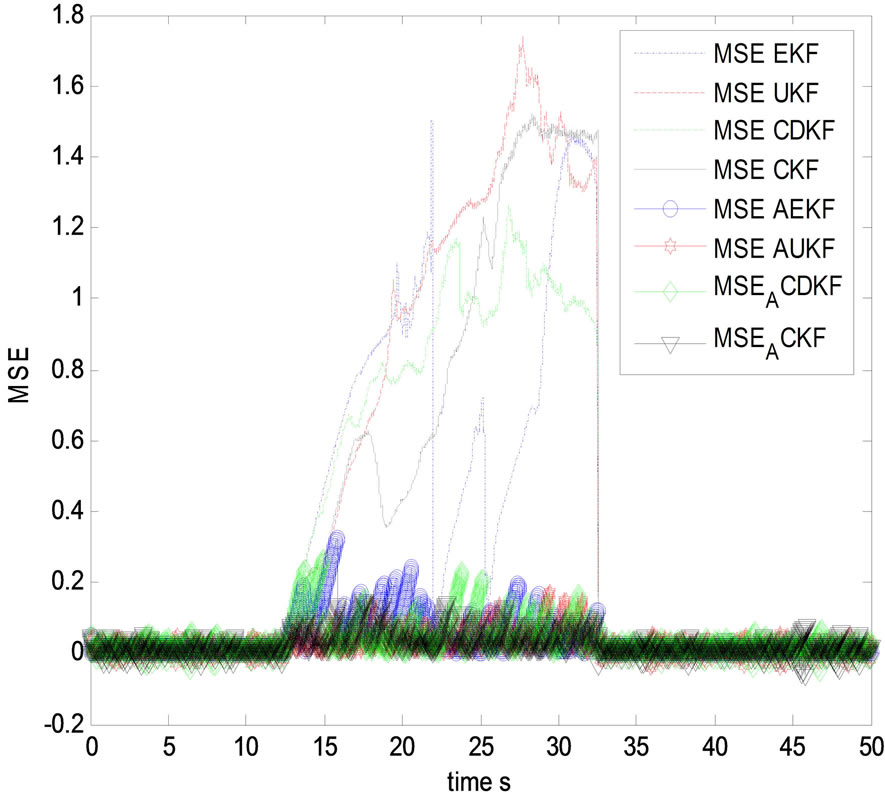
Figure 15. MSE pitch angle estimation in degree.

Figure 16. MSE pitch angle estimation in degree zoom.
simulated and activated between 13 s and 32 s. For the first part of simulation in normal flight conditions,

Figure 17. MSE roll angle estimation in degree.

Figure 18. MSE roll angle estimation in degree zoom.

Figure 19. MSE down velocity estimation (m/s).
between 0 and 13 s, it is possible to observe that all filters, classical and adaptive are superposed and present the same accuracy and convergence curve. This is logic re-
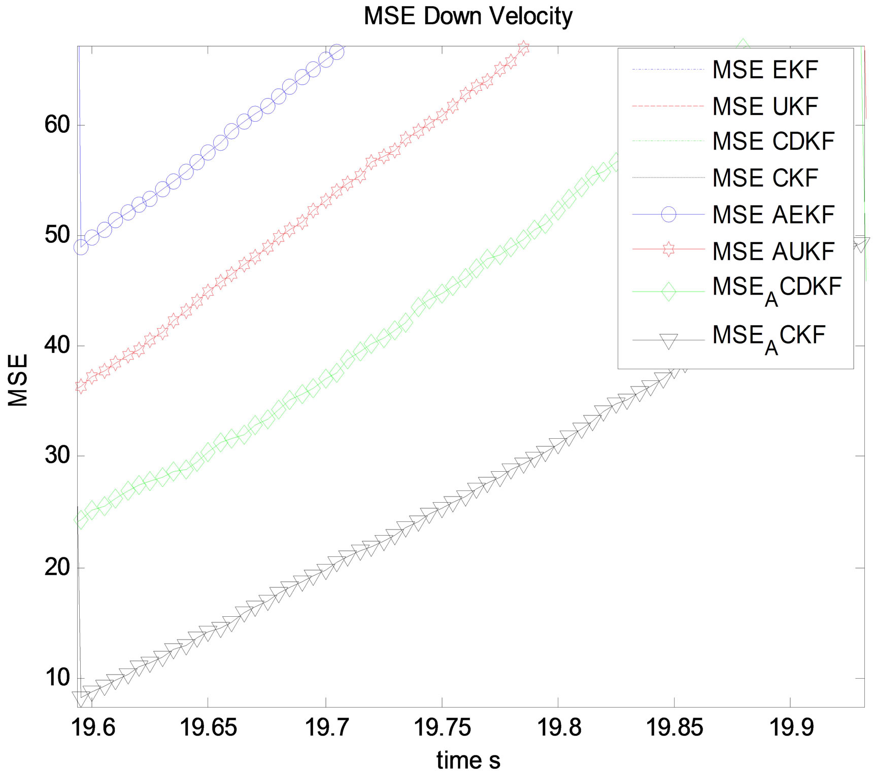
Figure 20. MSE down velocity estimation (m/s) zoom.

Figure 21. MSE east velocity estimation (m/s).

Figure 22. MSE east velocity estimation (m/s).
sults due to unuseful innovation based adaptive fading factors used to improve the accuracy of filtering algo-

Figure 23. MSE east velocity estimation (m/s) zoom.

Figure 24. MSE north velocity estimation (m/s).

Figure 25. MSE north velocity estimation (m/s) zoom.
rithms during outlier period. It is very interesting to observe the clear part of all figures which describes clas-

Figure 26. MSE vertical position estimation (m/s).

Figure 27. MSE vertical position estimation (m/s) zoom.
sical non linear filters EKF, CDKF, CKF and UKF without any adaptation, except for velocity estimation which in that case, UKF performs CKF in its non adaptive forms during outliers. This is an unexpected result between UKF and CKF. In this precise situation, UKF has better accuracy than CKF which is not usual in previous study and experiments in the field of data fusion. This is considered as a interesting novel result. As for EKF and CDKF, it is possible to observe too an additional interesting result, CDKF RMSE is less accurate than EKF RMSE during outlier period for velocity estimation which means that GNSS outliers affect more the CDKF covariance estimation than the EKF computation.
It is then possible to distinguish a classification of filters which is for most states estimation according the accuracy and convergence of filters: EKF, CDKF, UKF, CKF during outliers. It is very interesting to observe in the second curves of the adaptive filters the clear part of all figures which describes adaptive non linear filters AEKF, ACDKF, AUKF and ACKF, ACKF performs all adaptive ASPKF and AEKF during outliers. It is clear that ACKF maintain RMSE close to the minimum variance which is not the case for AUKF, ACDKF and AEKF, those algorithms present some impulsive errors during outliers even with innovation based adaptive fading factor. This is the proof that CKF after modification of its covariance and mean estimation presents a superior accuracy and stability of convergence comparing with modified SPKF and EKF. It is also clear that ACKF performs AUKF, ACDKF and finally AEKF. The last figures of position estimation, it is possible to observe the RMSE of ACKF, ASPKF and AEKF during outliers, and it is clear that for this linear state, non linear filters are non adequate only ACKF provide a good results between 9 s and 32 s. It is then possible to generalize the observation that all transformed filters AEKF, AUKF, ACDKF and ACKF outperform their classical algorithms EKF, UKF, CDKF and CKF respectively. This means that the solution we propose is a good alternative to GNSS outliers in IMU/GNSS data fusion.
6. Conclusion
The design of non linear adaptive filters and the associated data fusion based on EKF, SPKF and CKF were deeply studied for MEMS IMU/GNSS sensor fusion during satellite positioning outliers. Based on the innovation fading factor, 04 non linear filtering approaches EKF, KF, CDKF and CKF were modified using this fading factor for covariance and mean estimation during GPS/ LONASS outages. By the way, several solutions were proposed and ameliorated the accuracy and the time of convergence of each modified filtering algorithm. However according the RMSE criteria, Cubature Kalman Filter CKF during outliers demonstrated some limitation to perform Unscented Kalman Filter UKF in its non adaptive form. Finally, adaptive fading CKF demonstrated a large superiority in estimation accuracy and in its stability comparing with other filtering classes—adaptive EKF, adaptive UKF and adaptive CDKF.