Genetic Algorithm Based Node Deployment in Hybrid Wireless Sensor Networks ()
1. Introduction
A Wireless Sensor Network (WSN) is a distributed system which is composed of tiny, low-cost, battery-operated sensor nodes that collaborate together for the purpose of achieving certain task such as environment monitoring and object tracking [1]. Depending on the required application, the sensor nodes are responsible for sensing, computation and communication tasks. The sensing task is usually configured in each node; therefore the sensing attribute is considered a key factor in designing WSNs.
One of the key points in the design stage of a WSN that is related to the sensing attribute is the coverage of the sensing field. In the literature, the coverage problem in WSNs has been addressed either as target coverage or area coverage [2]. While area coverage protocols are designed to maximize the area of the sensing field that could be covered, target coverage, on the other hand, assumes that the sensing field is divided into targets. Therefore, the main objective of the target coverage protocols is to maximize the number of targets that could be covered in the field.
The coverage issue in WSNs depends on many factors, such as the network topology, sensor sensing model, and the most important one is the deployment strategy that is used to distribute or throw the sensor nodes in the field [3]. The sensor nodes can be deployed either manually based on a pre-defined design of the sensor locations, or randomly by dropping them from an aircraft. Random deployment is usually preferred in large scale WSNs not only because it is easy and less expensive but also because it might be the only choice in remote and hostile environments. However, random deployment of the sensor nodes can cause holes formulation; therefore, in most cases, random deployment is not guaranteed to be efficient for achieving the required objective in terms of the coverage [2].
In order to overcome the problem of holes formulation after initial deployment of the sensor nodes in the sensing field, an efficient algorithm that would maximize the covered area or targets should be employed. According to the application, the sensor nodes might be stationary, mobile, or hybrid in which some of the nodes are static and the others are mobile. In WSNs where all nodes are stationary, the area of the sensing field and the number of sensor nodes are small, coverage can be maximized by manually deploying additional nodes to the initially deployed ones. However, in large scale WSNs where human intervention is not possible or when the sensing filed is hostile, random deployment is the only choice.
In random deployment, the holes formulation problem might be reduced or eliminated after initial deployment using one of two approaches. In the first approach, if all sensor nodes are mobile, then an efficient algorithm should be designed such that the coverage is maximized while at the same time the moving cost of the mobile nodes is minimized. In this case, the mobility feature of the nodes can be utilized in order to maximize the coverage. After the initial configuration of the mobile nodes in the sensing field, an efficient algorithm such as potential field algorithm or virtual force algorithm can be employed for the purpose of relocating the sensor nodes [4,5].
In the second approach, if the sensor nodes are hybrid in which some of the nodes are stationary and the other are mobile, an efficient algorithm should be employed in order to find the number and locations of the mobile nodes that should be added after the initial deployment of the stationary nodes. One of the algorithms that can be employed is a genetic algorithm (GA) which is used to find an optimal or near optimal solution for optimization problems [6]. A little research in the field of WSNs has used and employed GA to search for an optimal number of sensor nodes that can be added after the initial node deployment in order to maximize the coverage.
In this paper, we propose an approach that exploits the movements of some nodes for eliminating the holes which would be formulated after the initial deployment of the sensor nodes. Our approach uses GA in order to determine the minimum number of mobile nodes that should be used in addition to the previously deployed stationary nodes such that the coverage of the monitored area is maximized.
This paper is organized as follows. Section 2 discusses the operation of the GA. Section 3 presents the related work. Section 4 discusses the assumptions and the components of the proposed approach. Section 5 presents simulation experiments and discusses the results, and Section 6 concludes the paper.
2. Genetic Algorithm
A genetic algorithm is used to search for near optimal solutions when no deterministic method exists or if the deterministic method is computationally complex. GA is a population based algorithm (i.e.; it generates multiple solutions each iteration). The number of solutions per iteration is called population size. Each solution is represented as a chromosome and each chromosome is built up from genes. For a genetic algorithm of population size n, it starts with n random solutions. Then it chooses the best member solutions for mating to generate new solutions. The best generated solutions will be added to the next iteration while the bad solutions will be rejected. While the algorithm iterates its solutions, these solutions are improved up to a point where converge to a near optimal solution is achieved. Many factors should be taken into consideration when the genetic algorithm is used. The first factor is the representation of chromosome and genes because bad representation may result in slower convergence. Another important factor is the mechanism of producing new solutions from the old ones. The most popular mechanisms are crossover and mutation. The third factor is how to find a fitness function (i.e.; a method to evaluate the solutions) in order to accept or reject the solutions, and how to select the best members for mating.
In general, a genetic algorithm has four stages: population initialization, evaluation of fitness, reproduction and termination. Initialization is the process of creating initial random solutions, which can be done by setting genes to random values. In the initialization process, n chromosomes are created as the first generation of solutions. After the initialization, each chromosome fitness (i.e.; solution goodness) is evaluated using the fitness function.
Reproduction process has four steps: selection, crossover, mutation, and accepting the solution. In the selection step, the fittest members in the current population are selected in order to reproduce new solutions. However, less fitness members will have also a chance to be selected. The selection step can be implemented by many mechanisms such as the rollet wheel method. This selection will be performed on two chromosomes to reproduce two new chromosomes each time. After selecting the chromosomes, a crossover operation is performed by selecting a random point in chromosomes and exchanging genes after this point. Crossover may be stuck in local optima. To overcome this problem, a tie breaker is needed which can be achieved by using mutation operation where a gene is selected randomly and its value is changed.
A widely used representation for genes is bits where each gene is represented by a bit. In this case, mutation is done by flipping a bit randomly in the chromosome. After crossover and mutation, two new chromosomes are reproduced. The final step is accepting these two chromosomes to be in the new population. Typically, the new chromosomes are accepted if they are better than their parents.
Termination is the last step in the genetic algorithm. Usually, the iteration of the genetic algorithm is stopped when a certain criterion is met. The most widely used stopping criterion is the number of iterations. When a predefined number of iterations are satisfied, the genetic algorithm is terminated.
3. Related Work
Several research works have addressed the node deployment problem to achieve maximum coverage in WSN. For random node deployment, these works considered WSNs that consist of mobile sensor nodes [4,5,7,8] or that contain both static and mobile nodes [9-12].
For mobile sensor networks, several approaches have been proposed. Voronoi diagrams were used in [7] to find the uncovered areas and determine the positions where the nodes can move. In [4], a potential field-based approach was proposed, in which a repelled force is generated between the obstacles and sensor nodes and among the nodes themselves, in order to evenly distribute the nodes in the field. A virtual force algorithm was proposed in [5] that uses both pulling and pushing force among the nodes. In [8], simulated annealing was used to find near optimal solutions for nodes placement that maximize the coverage of the area of interest.
On the other hand, several works have considered both static and mobile nodes in WSN. In [9], a bidding protocol was proposed, in which the static nodes are utilized as bidders and a number of mobile nodes move accordingly to satisfy the coverage requirements. In [10], a distributed protocol was proposed that considers the different sensing capabilities of the nodes using realistic sensing coverage model. In this protocol, the static nodes determine the uncovered areas using a probabilistic coverage algorithm and the mobile nodes move accordingly using virtual force algorithm. In [11], several approaches were proposed based on virtual force algorithm and particle swarm optimization. The obtained solutions were analyzed for better deployment in the region of interest. Recently, a biogeography-based optimization algorithm was proposed in [12] to maximize the coverage area of the network.
Genetic algorithms have also been used to solve the problem of optimal node deployment. While most of the proposed solutions have focused on deterministic node deployment [13-18], few works have been done in case of random node deployment [19-22]. In random deployment, genetic algorithms are applied to determine near optimal positions for additional mobile nodes in order to maximize the coverage. In [19], a force-based genetic algorithm was proposed, in which the mobile nodes utilize the sum of the forces used by the neighbors to choose their direction. In [20], a multi-objective genetic algorithm running on a base station was used. The base station determines where the mobile nodes can move to maximize the coverage and minimize the travelled distance. In [21], a cluster based WSN was considered and a genetic algorithm was used to find the best positions for the cluster heads that cover the maximum number of nodes and hence maximizing the area coverage. In [22], Voronoi diagrams were used to partition the field into cells and a genetic algorithm was then applied to determine the best positions for k additional mobile nodes that maximize the area coverage inside each cell.
Unlike the above-mentioned genetic algorithms, this paper proposes a genetic algorithm that finds the minimum number of additional mobile nodes and the best positions for these nodes in order to maximize the overall coverage
4. Proposed Approach
In this section, we present our proposed approach. We first present the network assumptions and coverage model, and then we discuss the GA-based approach.
4.1. Network Assumptions
It was assumed that the sensor nodes are randomly deployed and equipped with GPS, and the base station node position is stationary. Furthermore, the number of sensor nodes that are initially deployed equals the number of nodes that are required to achieve full coverage as if these nodes were deterministically deployed. It was also assumed that few mobile nodes are available and can be used to repair the coverage holes after initial deployment of the stationary nodes.
4.2. Coverage Model
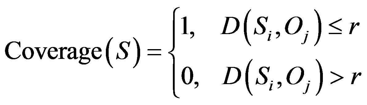
We assumed that each sensor node with a sensing radius r can cover an area of circular shape. We also assumed that a target object Oj can be detected by sensor Si if Oj is within the sensing range of Si. This can be represented using the binary model of sensor detection which is given by:
 (1)
(1)
where D is the distance between the target object being sensed Oj and the sensor node Si. The coverage function Coverage(S) equals 1 when the target object can be covered or sensed, otherwise it equals 0.
4.3. GA-Based Approach
The main objective of employing the GA in our approach is to maximize the coverage by reducing or eliminating the holes that are formulated after initial deployment of the stationary nodes. Figure 1 shows the pseudo code of the proposed GA algorithm. Assume that Si stationary sensor nodes are deployed randomly over a sensing field, and all the sensor nodes have the same sensing range which is represented as a circle with radius r. Then, the base station will run the GA after gathering the locations of the stationary sensor nodes in order to determine the
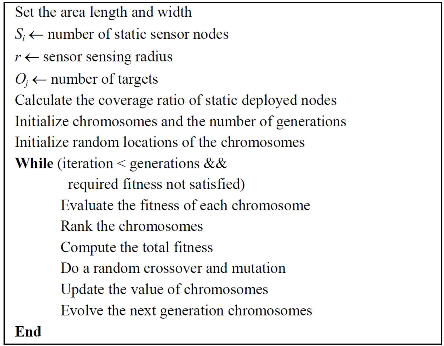
Figure 1. Implementation procedure of the GA-based optimization model.
number and locations of the mobile nodes as follow:
1) Chromosmes modeling: Each chromosome, as a solution in the GA, represents the location of a potential mobile sensor node in the sensing field modeled as (X, Y) point. The gens of each chromosome represent a binary digit that resembles the value of the location on the X and Y axises. For example, in order to represent a mobile node mapped to location (30,40), the corresponding chromosome is shown in
Figure 2" target="_self"> Figure 2. The size of the chromosome population is selected based on two factors: the area of the sensing field and the initial configuration of the network. For instance, if the area of the sensing field is 50 m ´ 50 m, the sensing radius of each node is 8m, and the number of deployed stationary nodes is 13 (i.e.; 50
2/(p×8
2) ≈ 13), then the proposed GA will start with population of 13 randomly generated chromosomes. Note that value 13 is selected in this case based on the assumption that 13 sensor nodes would cover the entire field as if they were deterministically deployed.
2) Fitness function: In GAs, an objective function is defined in order to evaluate the fitness of each solution to the corresponding objective. The formulation of the objective or fitness depends on the problem characteristics. The fitness function is used in order to choose the best fittest chromosomes for the purpose of reproduction of the next generated solutions by the GA. The fitness function in our model defines the mutually exclusive coverage ratio of each chromosome. That is, the fitness function calculates the maximum number of covered targets by each mobile node if and only if these targets are uncovered by other mobile or static nodes. This property of the fitness function prevents the overlapping redundancy among the coverage regions of the deployed mobile nodes and forces each mobile node to cover only a distinct region. The fitness function is given by:
X-location Y-location
|  0 |
1 |
1 |
1 |
1 |
0 |
1 |
0 |
1 |
0 |
0 |
0 |
Figure 2. Chromosome representation of sensor location (30, 40).
 (2)
(2)
where F(MSi) is the fitness of mobile node i (MSi) which calculates the coverage as a function of the targets it covered, given that the target object Oj is not covered by any stationary node or other mobile nodes. In Equation (2), Sc is the coverage of initially deployed stationary nodes and F(MS/i) is the coverage of any mobile node except mobile node i.
To choose the fittest species for mating in the next generation, we defined a fitness ratio for each mobile node as a function of its coverage and the total number of targets, which is given by:
 (3)
(3)
We also defined a function that measures the total coverage of the network at each GA generation. This function is defined as an accumulation of the coverage of the static nodes and the generated mobile nodes, and is given by:
 (4)
(4)
3) GA operators: We used the fitness ratio calculated in Equation (3) as a measure for ranking the chromosomes and then performing parent selection according to the ratio participated by each chromosome in the fitness function. The chromosomes with higher ranking have a higher probability to become parents and perform reproduction of new individuals than others with smaller ranking. This property must be maintained in order to increase the improvement ratio at each generation of the GA. With high probability, a crossover operation is performed between a pair of parent chromosomes in order to create two offspring. In the crossover operation, the crossover point is choosed randomly where two parent chromosomes are selected, and then the chromosome parts are exchanged after that point. The sequence of selection and crossover operations may lead to a state where all chromosomes are identical and thus the algorithm stops creating new individuals. This may prevent the average fitness improvement and thus trapping into a local optimum. To solve this problem, a mutation operation, with low probability, is applied to toggle the randomly selected gene on the chromosomes.
4) Termination condition: We defined the termination condition of the applied algorithm in terms of the number of generations and coverage ratio perspectives. That is, the algorithm terminates either when the required network coverage ratio is reached or when the algorithm reaches the specified number of generations.
5. Performance Evaluation
In this section, the performance of the proposed algorithm is evaluated in terms of the amount of coverage (coverage ratio), degree of coverage (k-coverage), and number of additional mobile nodes. Moreover, the effect of the number of randomly deployed static nodes and the sensing ranges on coverage and number of additional mobile nodes were investigated.
Two simulation experiments were conducted for performance evaluation. In the simulation environment, it was assumed that the sensor nodes were randomly deployed and the targets were uniformly located in a 200 m ´ 200 m sensor field. In the first experiment, the number of deployed static nodes varies from 100 to 200 to cover 625 targets, whereas the sensing ranges of all nodes are fixed to 12 m. In the second experiment, the number of deployed static nodes is fixed to 100, while the sensing ranges vary from 10 m to 20 m. In each experiment, the coverage ratio, k-coverage, and number of additional mobile nodes were measured before and after applying the proposed algorithm.
5.1. Effect of Number of Static Nodes
Figure 3 shows the coverage ratio when the static nodes are randomly deployed and after adding the mobile nodes to the network. As shown, the coverage ratio increases as the number of deployed static nodes increases. The coverage of the static nodes alongside the additional mobile nodes clearly outperforms the case of random deployment of the static nodes as the additional mobile nodes are located into regions where targets are not covered by the static nodes.
Figure 4 shows the k-coverage when the static nodes are randomly deployed and after adding the mobile nodes to the network. For both cases, it is shown that as the number of nodes increases, the k-coverage increases. This is because the static nodes in both cases are randomly deployed and it is very likely that the coverage among these nodes is overlapped, hence the targets would be covered by more sensor nodes as the number of static nodes increases.
Figure 5 shows the number of additional mobile nodes versus the number of randomly deployed static nodes. As shown, the number of mobile nodes decreases as the

Figure 3. Comparison of coverage ratio for different number of deployed nodes.
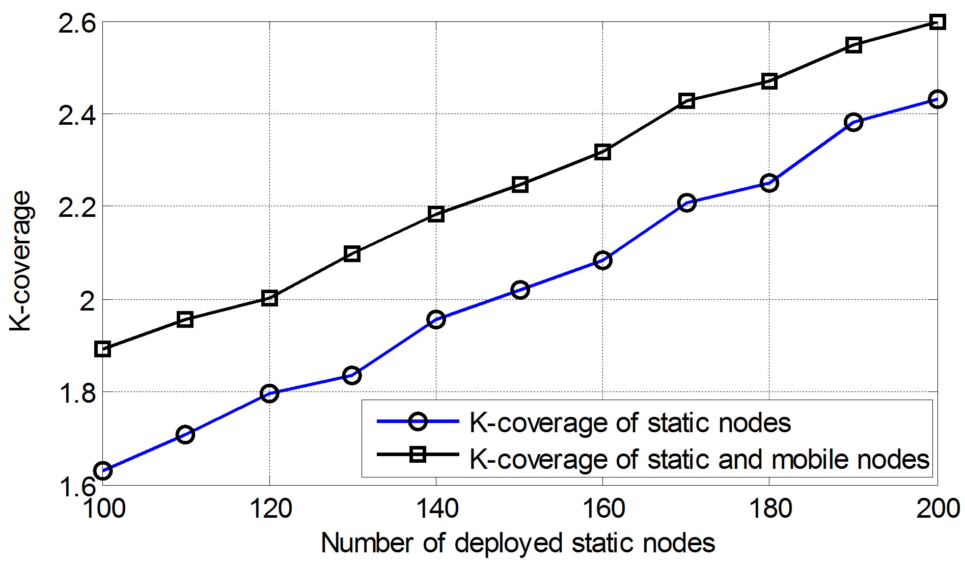
Figure 4. Comparison of k-coverage for different number of deployed nodes.

Figure 5. Number of additional mobile nodes versus number of static nodes.
number of static nodes increases. This is because more targets would be covered as the number of static nodes increases and hence less mobile nodes would be added to increase the coverage ratio.
5.2. Effect of Sensing Range
Figure 6 shows the coverage ratio when the static nodes are randomly deployed and after adding the mobile nodes as a function of the sensing ranges. It is shown that the coverage ratio increases as the sensing radii of the deployed nodes increase, since sensor nodes with larger sensing range can cover more targets than that with smaller range. The coverage of the static nodes along with the additional mobile nodes clearly outperforms the case of random deployment of the static nodes as the additional mobile nodes are located into regions where targets are not covered by the static nodes.
Figure 7 shows the k-coverage when the static nodes are randomly deployed and after adding the mobile nodes as a function of the sensing ranges. As shown, the kcoverage increases as the sensing radii of the deployed nodes increase. This is because the coverage among sensor nodes with large sensing range is very likely to overlap, and hence more targets would be covered by multiple nodes.