Cluster Analysis Assisted Float-Encoded Genetic Algorithm for a More Automated Characterization of Hydrocarbon Reservoirs ()
1. Introduction
Borehole geophysical measurements are extensively used in hydrocarbon exploration for collecting high resolution in-situ information about subsurface geological formations. Well-logging data measured by different physical principles are recorded along depth in the form of well logs [1]. The primary aim of the interpretation of observations is the lithological separation of the succession of strata and the estimation of thicknesses and petrophysical properties of formations (such as porosity, water saturation, mineral content, permeability, etc.) for the calculation of oil and gas reserves. The most advanced tools of well log analysis are based on geophysical inversion methods. By assuming a petrophysical model, one can calculate theoretical well logs, which are compared to real ones measured in the borehole. The initial model is progressively refined in an iteration procedure until a proper fit is achieved between the predictions and observations. The estimated model obtained in the last iteration step is accepted as the solution of the inverse problem that represents the most probable geological structure. The mathematical basis and computer implementation of traditional well-logging inversion methods, which solve the inverse problem depth by depth separately, can be found in [2-4]. The positions of layer-boundaries cannot be extracted from the local data set by this inversion method. Instead they are picked out on the lithological logs manually. A novel inversion method that inverts a data set of a greater depth interval to estimate the variation of petrophysical parameters and thicknesses along a borehole was developed by the Department of Geophysics, University of Miskolc. The inversion methodology named interval inversion has been applied to solve several hydrocarbon exploration problems [5-9].
Multivariate statistical methods are proven to be powerful tools in formation evaluation [10]. Regression, factor and cluster analysis are widely used to find correlations between petrophysical variables, to reduce problem dimensionality or explore non-measurable background variables as well as to separate observed data into distinct groups of different lithological characters. The principles of clustering techniques are detailed in [11], to which a variety of petrophysical applications can be found in the literature, e.g. in [12-15]. In this study, we apply the hierarchical form of cluster analysis to separate nearly homogeneous beds of shaly-sand sequences on a lithological basis. This technique is able to specify the coordinates of layer boundaries in an automatic procedure, which are then used as input for solving a global optimization-based interval inversion procedure. The workflow enables a fast and automatic estimation of layer-boundaries and petrophysical parameters to provide the log analysts and reservoir engineers with accurate and reliable information for planning the exploitation of hydrocarbon fields.
2. Theory of Interpretation Method
2.1. Well-Logging and Inversion
Several books deal with the basics of well-logging surveying and interpretation methods, among them many was written chiefly for petroleum geologists [16,17]. The classification of well logs can be made by parameter sensitivities [18], which in this particular case inform how the data are influenced by the petrophysical parameters, separately. Accordingly, three main groups of measurements can be distinguished, i.e. lithology, porosity and saturation sensitive logs.
In hydrocarbon exploration relatively high cost measurements are made to increase the probability of finding an economically valuable oil/gas field. Normally, a field data set consists of natural gamma-ray intensity (GR), spectral gamma-ray intensity such as potassium (K), thorium (TH), uranium (U), and spontaneous potential (SP) data (lithology logs). Porosity logs comprise formation density (DEN), neutron porosity (NPHI) and acoustic traveltime (AT) data. Resistivity tools measure the formation resistivity with different penetration depth from the borehole wall. In this study, true resistivity (RT) log is applied that represents the corrected resistivity of the part of formation not invaded by the drilling mud (saturation log). The observed data are inverted to derive petrophysical properties of formations such as effective porosity, water saturation at different penetration depth, mineral volumes, shale content and permeability that cannot be measured directly, but necessary for the calculation of hydrocarbon reserves. Since the measured data can be related to petrophysical parameters by probe response equations [5], thus the latter can be estimated by an iterative inversion procedure. The principles of geophysical inversion and related issues are detailed in [19]. Inversion methods are preferred as they use all suitable logs instead of one or two logs to reduce the estimation error of petrophysical parameters. To further increase the performance of inverse modeling as much good quality prior information as possible should be given and proper optimization strategy must be posed when they are applied.
2.2. Local Inverse Modeling
Let m be the column vector of model parameters such as porosity (POR), water saturation in the flushed zone invaded by mud filtrate (SX0), water saturation of undisturbed formation (SW), shale volume (VSH), quartz content (VSD) in a given depth. Well-logging data types measured at the same measuring point are also represented in a column vector d(m). If we consider the data set listed in Section 2.1, an inverse problem with 5 unknowns and 9 data has to be solved in each depth. In this case, the overdetermination (data-to-unknowns) ratio is 1.8.
Theoretical (calculated) well-logging data are connected to the petrophysical model nonlinearly as d(c) = g(m), where g represents a set of probe response functions. Substituting the initial guess of model parameters to the empirically derived response equations one can calculate a local data set in the measuring point. The solution of the inverse problem is found at the minimal misfit between the observed and predicted data [19]. The Euclidean norm of the deviation between measured and calculated data vectors is applied as an objective function for the optimization
 (1)
(1)
where σk is the variance of the k-th well log depending on the probe type and borehole conditions (N is the number of applied probes). To optimize Equation (1), the Weighted Least Squares method (WLSQ) is used, where the actual model is gradually refined by m = m(0) + dm, where m(0) is the initial model and dm is the model correction vector. By introducing the diagonal weighting matrix Wkk = 1/sk2 (k = 1,2,…N) including data variances, the vector of model corrections in a given iteration step can be estimated by
 (2)
(2)
where G denotes the Jacobi’s matrix containing partial derivatives of data with respect to model parameters and dd is the difference between the measured and calculated data vector (T is the symbol of matrix transpose). The quality check of inversion results is based on the following connection between the uncertainties of observed data and model parameters [19]
 (3)
(3)
where covm and covd denote the data and model covariance matrices, respectively, and M is the generalized inverse matrix of the actual inversion method. The latter can be expressed with the proper combination of matrix G. If we know data variances from covd, Equation (3) gives the estimation errors of model parameters at the end of the inversion procedure. They are obtained from the main diagonal of model covariance matrix as sm,I = sqrt(diag(covmii)). For measuring the distance between the observed and calculated data the RMS error is normally used.
2.3. Genetic Algorithm-Based Interval Inversion
Linearized optimization methods work properly and quickly only when an initial model sufficiently close to the solution is available. However, in cases when poor prior information or rather noisy data is provided the WLSQ procedure can be easily trapped in a local minimum of Equation (1). To avoid localities a global optimization method such as Genetic Algorithm (GA) is used that searches the absolute extreme of the objective function. GA belongs to the class of evolutionary algorithms that solves optimization problems using the analogy of natural selection of living populations [20]. Nowadays the most preferred variant is the Float-Encoded GA that improves a model population represented by model parameters from the domain of real numbers in an iteration procedure [21].
In the population each individual has a fitness value representing its survival capability. During the genetic process the fittest individuals reproduce more successfully in the subsequent generations than those who have relatively low fitness. To achieve the best solution, the fitness function is maximized by using genetic operations in a random optimum-seeking procedure. From the point of view of well-logging inverse problem a petrophysical model has large fitness when the misfit is relatively small between the observed and calculated data. In well-logging inversion normally 30 - 100 model take part in the selection process. To reach the absolute maximum of fitness function a proper combination of genetic operators such as selection, crossover, mutation and reproduction is used (GA search in Figure 1). According to our experience after some tens of thousands generations (iteration steps) the fittest individual of the last generation can be accepted as the optimal petrophysical model. More details of the GA-based inversion procedure can be found in [5,9].
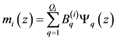
Local inversion methods (Chapter 2.2.) process barely more data than unknowns, where the accuracy of solution highly depends on the noise level of data and the initial guess of the petrophysical model. To increase the overdetermination of the inverse problem, we define a set of probe response functions as d(z) = g(m(z)), which is valid in a greater depth interval. In the response functions the data and model parameters are varying with depth. To discretize the depth variations of petrophysical unknowns we suggest a series expansion technique
 (4)
(4)
where mi denotes the i-th model parameter, Bq is the q-th expansion coefficient, Ψq is the q-th basis function, Qi is the requisite number of coefficients describing the i-th unknown. Basis functions in Equation (4) are known and arbitrarily chosen. For instance, in homogeneous layers a combination of heaviside functions (u) is advantageous to use as basis function. From one hand, using the basis function , each petrophysical parameter in the q-th layer (where
 ) can be described by one series expansion coefficient. On the other hand, we can introduce
 , Zq upper and lower depth coordinates of the q-th layer as unknown in the inverse problem [5]. For describing inhomogeneous intervals polynomial basis functions can be used [7]. The model parameter vector to be determined by inversion is m = [B,Z]T, where B and Z vectors contain all series expansion coefficients given in Equation (4) and layer-

Figure 1. Workflow of the GA-based inversion procedure.
boundary coordinates (or thicknesses) in the processed interval, respectively.
The fitness function of the GA process is inversely connected to the objective function of the well-logging inverse problem. We tested two types of fitness functions. The first one follows the idea of traditional inversion methods represented by the objective function in Equation (1)
 (5)
(5)
where P is the total number of measuring points. The minimization of the weighted least squares criterion in Equation (5) leads to optimal solution as well-logging data have different magnitudes and measurement units. The only weakness of weighting by variances is that we have to know standard deviations of all data types in each depth. In fact, the variances of data in most of the cases are not known (just from literature given for probe types), because normally we measure only once in a depth point. Our experience shows that an optimal solution can be given by normalizing the individual data differences by the measured data
 (6)
(6)
To compare the performance of the F1 and F2 based interval inversion procedures a four-layered petrophysical model was defined (Table 1). We calculated synthetic data by the exact model parameters (POR, SX0, SW, VSH, VSD). To synthetic well logs 5% Gaussian distributed noise was added to produce quasi measured data

Table 1. GA interval inversion results for synthetic case.
substituting real measurements. The input of the inversion procedure was a noisy well-logging data set includeing 1400 data (20 m processed length, 0.1 m sampling interval, 7 types of well logs).
Series expansion was developed for describing a layerwise homogeneous model. There were 20 unknowns against data, thus the overdetermination ratio (70) was almost 40 times higher than that of local inversion (Section 2.2.). In Equation (5) the standard deviations of data were calculated empirically for each data types layer by layer. For the characterization of misfit we used the relative data and model distances. The first measures the difference between the measured and calculated data, the latter quantifies the deviation between the estimated and (exactly) known model
 (7)
(7)
where m(e) and m(t) denote the estimated and target model, respectively (L is the number of layers, M is the number of model parameters). The outputs of inversion program runs in Table 1 show highly accurate estimation results. We let the search run till 15,000 generations in both cases (Figure 1). The inversion procedures were stable and the data distance of the solutions based on Equation (7) was around 5.1% (Figure 2(a)). The model distance for fitness function F1 was 0.85%, while that of F2 was 0.62% (Figure 2(b)). It was concluded that the application of both fitness functions led to the same (global) optimum. In case of F2 a faster convergence towards the optimum was found after iteration 1000, and a little higher retrieval accuracy was indicated as the relative improvement of model distance was 37% compared to the case of F1.
After defining a proper fitness function, the upper and lower boundaries of model parameters and the control parameters of genetic operators must be specified (specifying search domain in Figure 1). The optimal values of series expansion coefficients B are estimated by the GA-based interval inversion method, which are substituted into Equation (4) to produce the vertical distributions of petrophysical parameters. The determination of layer-thicknesses cannot be accomplished with local inversion methods. They have to be a priori known before starting a local inversion procedure. In interval inversion only the lower and upper limits of thicknesses are required that means a non-automatic processing step. To automate this phase, we use cluster analysis for producing the estimates of layer-thicknesses that can be treated

Figure 2. Convergence of interval inversion procedures.
either as constant or unknown in the interval inversion procedure.
2.4. Hierarchical Cluster Analysis
Clustering methods can be effectively used for the grouping of well-logging data in such a way that the N dimensional objects specified by data sets measured from given depths are more similar than others observed from different depths. From the point of view of our method, it is of great importance that objects connected to the same cluster define approximately the same lithologic character, while other clusters represent dissimilar ones.
Agglomerative clustering methods build a hierarchy from the observed objects by progressively merging clusters. At the beginning, we have as many clusters as individual elements. In the first step, the closest points are coupled together to form a new cluster. In each following step, the distances between objects are re-calculated and the procedure is continued until all elements are grouped into one cluster. In this study, we used the matrix of Euclidean distances as a measure of dissimilarity between the pairs of observed objects. During the procedure the distances between the elements of the same group are minimized while they are maximized between the clusters at the same time. During the reconnection of clusters we follow the Ward’s linkage criterion that minimizes the deviances of (xi-c), where xi is the i-th object and c is the centroid (average of elements) of the given cluster [22]. The result of cluster analysis is a dendrogram that shows the steps of clustering as it provides the hierarchy of clusters and the connections between them at different distances.
We use cluster analysis as a preliminary data processing step before inverse modeling (Figure 1). The input of clustering is the complete data set originated from the logged interval. By finding the similarities between raw data the objects are grouped into clusters. The log of clusters correlates well to the lithology variation along a borehole. The change in the group number of clusters appearing on the log gives the positions of layer boundaries, which can be read automatically by computer processing. The estimated layer-boundary coordinates as important a priori information for constructing the starting model serve as input for the interval inversion procedure.
3. Hydrocarbon Field Application
We tested the inversion method on a borehole geophysical data set measured from a Hungarian hydrocarbon well (Well No. 1). We used GR, K, U, TH, DEN, NPHI, AT, RT logs as input for the interpretation procedure. In the processed interval a sedimentary complex made up of four unconsolidated shaly-sand beds is found. The crossover effect between DEN and NPHI logs confirms the presence of gas in the porous and permeable formations. According to the workflow in Figure 1, at first a simultaneous cluster analysis of the 8 logs was performed. We specified three lithological categories: shale, shaly sand and sand. At this stage of interpretation, this resolution is enough for finding the layer-boundaries, because the relative volumes of rock-forming sand and shale can be estimated later in the inversion processing phase. For measuring the distance between the observed objects we used a standardized Euclidean distance, where each datum in the sum of squares is inversely weighted by the sample variance of that data type. We assigned leaf node numbers for each object in the original data set, where some leaf nodes correspond to multiple objects (Figure 3(b)). We created the hierarchical cluster tree of 30 objects by using the Ward’s linkage algorithm (Figure 3(a)).
On the dendrogram 3 clusters can be discriminated at distance 15. The 3D crossplots of clustered well-logging data can be seen in Figures 4-6. The plots give useful information about some site-specific constants for calculating wellbore data in the straightforward modeling phase (well-logging data prediction in Figure 1) as values of physical properties of rock constituents (sand, shale) must be specified in probe response equations. For instance, the neutron porosity of sands (15%) and shale (26%) or the natural gamma-ray intensity of sand (40 API) and shale (110 API) can be estimated for the given hydrocarbon zone (Figure 5).
The log of the group numbers of clusters is useful to separate three types of formations (sand reservoir, shale, shaly-sand reservoir). The layer-boundaries are normally picked out at the places of inflection points on the GR

Figure 3. Result of cluster analysis in Well No. 1.

Figure 4. Clustered spectral gamma-ray intensity log data in Well No. 1.
curve. These depths are well indicated by abrupt changes in cluster log. In the given example, the layer-boundary coordinates were found at 4 m, 8.4 m, 9.6 m, 16 m. We set these coordinates fixed, then petrophysical parameters were determined by interval inversion.
In the interval inversion phase, we applied a series expansion of model parameters (POR, SX0, SW, VSH, VSD) for a combination of homogeneous and inhomogeneous layers. Until the depth of 9.6 m the 3 layers can be treated as homogeneous ones. Below 10 m the 2 statistically located layers can be coupled as they belong to the same hydrocarbon reservoir. For the first 3 layers unit step functions, for the rest ones fourth-degree power functions were used as basis functions in Equation (4).

Figure 5. Clustered neutron, acoustic and natural gammaray intensity log data in Well No. 1.

Figure 6. Clustered bulk density, resistivity and natural gamma-ray intensity log data in Well No. 1.
The standalone GA procedure is very time-consuming. For decreasing the CPU time of the inversion procedure we implemented a hybrid optimization technique that is based on the successive combination of global and linearized optimization methods [8]. We start the procedure with global optimization (GA) that performs a random search in the parameter space avoiding the local maxima of F2 in Equation (6). Then, after some 200 generations, in the near vicinity of the absolute maximum, we change for a faster linear optimization method (Figure 7). We used the Damped Least Squares (DLSQ) method for the minimization of objective function E* = -F2 in the sec-

Figure 7. Convergence of GA + DLSQ interval inversion procedure in Well No. 1.
ond phase with applying proper damping factor to avoid big skips from the optimum [19]. This method both accelerates the rate of convergence of the inversion procedure and gives the estimation errors of model parameters as the Jacobi’s matrix is calculated by Equation (3) at the end of the procedure.
The petrophysical parameters and their estimation errors are listed in Table 2. In the 4th layer, the depth coordinates were properly transformed into the range of 0 and 1 for the polynomial approximation, where C0 denotes the coefficient of the 0th power exponent of depth coordinate as independent variable. The inversion results are highly accurate according to the values of estimation errors. This is because of the high overdetermination of the inverse problem. For further increasing the overdetermination, parameter VSD in the 4th layer was calculated by the physical constraint . The measured logs and inversion results are in Figure 8. The log of the group numbers of clusters is represented in track 6, while the inversion estimates are in tracks 7 - 8, where the relative volume of water, movable and ireducible hydrocarbon, pore space, shale, sand can be analyzed visually. In the 4th layer, gas is accumulated at the top of the reservoir, while the denser water is situated underneath. The amount of shale is increasing with depth in the lowest formation.
4. Conclusions
The ever-increasing claim of oil industry lain to highly reliable petrophysical information requires advanced data processing techniques. In the paper, a quick automated inversion method was shown for the interpretation of borehole geophysical data. The cluster analysis assisted joint inversion method is highly accurate (assured by great amount of overdetermination), automatic (automated layer boundary and petrophysical model estimation), robust and adaptive (evolutionary algorithm phase)
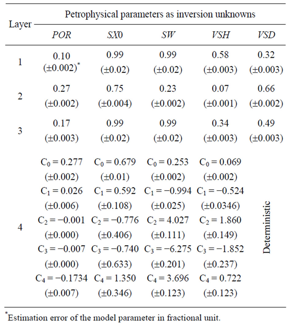
Table 2. GA interval inversion results in Well No. 1.
and fast (hybrid optimization technique; simultaneous inversion processing of data from the logged interval instead of one point).
The inversion method is not fully automatic, where the supervision of the log analyst cannot be discarded. To achieve a good and unique solution, the prior geological and geophysical information must be built-in by the user properly (chose of site specific constants and response equations in different hydrocarbon zones). Moreover, in case of the global optimization phase (GA), some experience is needed to set the combination and control parameters of genetic operators and to decide when it is possible to switch over to linear optimization. As a speciality of the interval inversion method, the basis functions of series expansion can be chosen arbitrarily. The optimal set of basis functions to be in use depends on the variation of lithology and pore fluids along a borehole. A trade-off must be taken between the vertical resolution (number of unknowns) and stability (uniqueness) of the inversion procedure as they are inversely proportional. Usually, this is the most important question from the point of view of constructing an inversion method. To increase the overdetermination of the inverse problem, it is important to search for such parameters that can be fixed during the inversion procedure. The cluster analysis-based interval inversion method helps to find lithological similarities in the data set, which leads to constrain the inversion process with reliable site constants and layerthicknesses. This can reduce the uncertainty and ambiguity of inversion estimates. In the future, we are planning

Figure 8. Processed well logs and result of cluster analysis assisted interval inversion procedure.
to find technical solutions to reach even better spatial resolution of petrophysical properties with preserving stability by using orthogonal polynomial series expansion along the entire logging interval and further develop the multiwell applications of the presented inversion method.
5. Acknowledgements
The described work was carried out as part of the TÁMOP-4.2.2/B-10/1-2010-0008 project in the framework of the New Hungary Development Plan. The realization of this project is supported by the European Union, co-financed by the European Social Fund. N. P. Sz. as the leading researcher of project no. PD 109408 thanks to the support of the Hungarian Scientific Research Fund. M. D. as the leading researcher of project no. K 109441 thanks to the support of the Hungarian Scientific Research Fund. N. P. Sz. thanks to the support of the János Bolyai Research Fellowship of the Hungarian Academy of Sciences. We thank the long-term co-operation to the Hungarian Oil and Gas Company.