Forecasting the Convergence State of per Capital Income in Vietnam ()
1. Introduction
Suppose that we observe an economic variable  being a stochastic process dependent on parameter
  (time),
  (space) with considered area X. Observations
  at time (period)
 are known, and we consider following convergent conception of economic variable
  (t is unlimited over time) as the convergence of function
  for finite value
  (called “convergence state”) at sub-regions (province)
 (1)
(1)
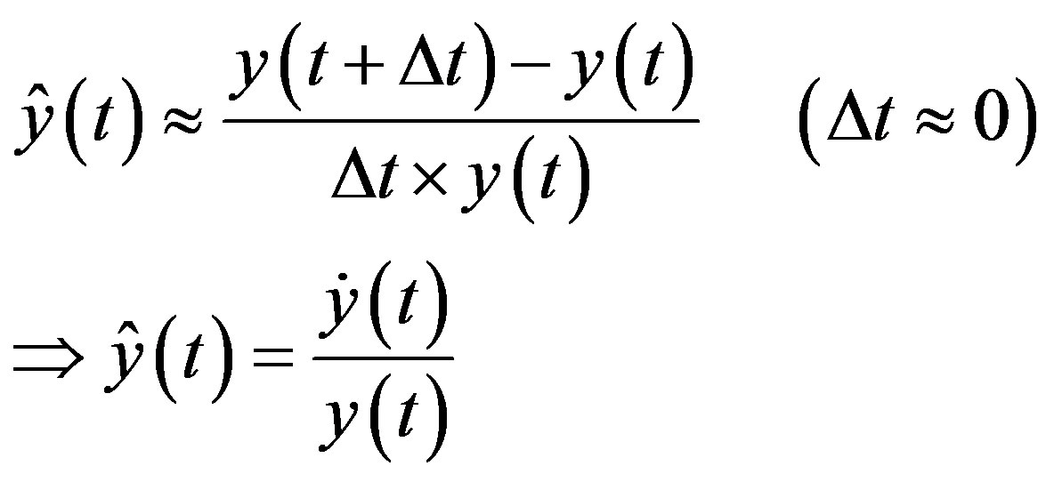
Growth coefficient  of the economic variable reveals variable rate (the variable level of a unit), variable
  in a unit of time at time
 :
:
 (2)
(2)
For the model (1) with  assigned to income or productivity, the convergence in income and productivity is among the most-receiving attention economic issues in recent years. There is an urgent need for research on the convergence due to its theory and practical value. Theoretically, analyzing the convergence can help to distinguish the different growth theories based on its forecast on economic growth. Otherwise practically, convergence researching can contribute to planning and evaluating the provincial policy measures at time when the economic differences between sub-regions in a region are profoundly gained. Therefore, convergence researches are conducted widely between many nations and regions. Many authors focused on the convergence in income, however, studying the convergence in GDP according to regions also provides many such important information. Globally, implementing the Barro recurrent in convergence researches was mentioned in many countries but only the information of the initial and final stages of the researches was analyzed. Exploiting this information at all stages was not set forth yet. In Vietnam, as the authors recognized, the implementation of classic Markov method in examining the convergence in income per capita and productivity, growth rate hasn’t been studied yet. Therefore, this study is designed to introduce a new method to Vietnam’s economic growth research at the region levels.
This paper aimed to evaluate the convergence level in provinces of Vietnam (sub-regions) based on income per capita which is examined through their data on GDP, population and manpower in the period 1990-2007.
The idea of convergence in economics (also sometimes known as the catch-up effect) is the hypothesis that poorer economies’ per capita incomes will tend to grow at faster rates than richer economies. As a result, all economies should eventually converge in terms of per capita income. Developing countries have the potential to grow at a faster rate than developed countries because diminishing returns (in particular, to capital) are not as strong as in capital-rich countries. Furthermore, poorer countries can replicate the production methods, technologies, and institutions of developed countries.
In economic growth literature, the term “convergence” can have two meanings. The first kind (sometimes called “sigma-convergence”) refers to a reduction in the dispersion of levels of income across economies. “Beta-convergence” on the other hand, occurs when poor economies grow faster than rich ones. Economists say that there is “conditional beta-convergence” when economies experience “beta-convergence” but are conditional on other variables being held constant. They say that “conditional beta-convergence” exists when the growth rate of an economy declines as it approaches its steady state.
2. Theoretical Basis
2.1. Economist View of Considered Approaches
Generally, convergence results from neoclassical growth theory where for certain set of economies, their economic growth is infinitively unstable and lessening at the end, and their speed is likely to come to stationariness as production function drives downward performances by capital size. If these groups of economics have similar economic structures, they would converge at a same stable condition, narrowing the income gap. At that case, an absolute convergence occurs. However, in the case the economics see differences in their structures, they witness diverse “stable conditions” and uncertain decrease in income-gap, which is called conditional convergence. Differences in their “stable conditions” will be partially explained in some additional variables (see [1]). This paper only focuses on absolute convergence.
When analyzing a standard convergence, researchers investigate (the presence of) the convergence which presents a declining income-gap and the convergence displaying whether the poor nations witness a faster economic growth than the developed ones. It’s said that absolute convergence takes place when initial income and its later development have a negative relationship. From this theoretical economic point, the classical Barro recurrent models are widely implemented (see [1-3]), it’s reckoned that: in the observed time , the growth pace of economic variable
  is defined as:
Barro model
 (3)
(3)
With  is the initial value of economic variable;
  server as parameter which are estimated based on the correspondent regression equations:
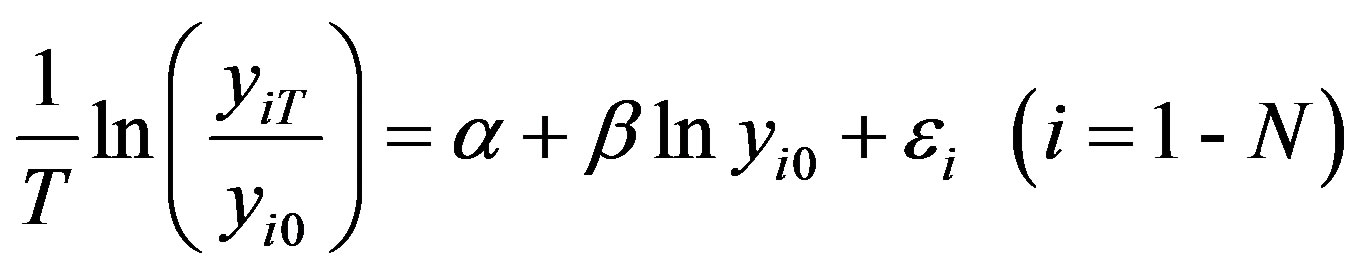 (4)
(4)
(Barro regression equation)
With  -observed error,
 —sub-region number (provinces, cities, localities…) survived in
  (nations, zones….);
  and
and  is the observed value in sub-region
  of economic variable at the starter
  and
and  in the studied time
 . After estimating the parameters in the above recurrent formula, the Neoclassical economics paradigm is employed to provide sufficient signs for variable
  to converge
 . Nevertheless, before this sign is used (when economic variable presents for income or productivity), it’s a must to check the form of Cobb-Duglass in the function for manufacturing or the concave condition of combined function for manufacture. This can’t always be achieved, especially in the Barro recurrent when only the information of its initial and final steps are studied
 . Additionally, these mentioned sufficient signs can’t help the researchers come to a certain conclusion about the inability of convergence of economic variable
 . Therefore, the group of authors will introduce a new method named “expanded Barro recurrent method” in the next 2.2 to surmount this defect. A second method: Markov method (see [4,5]), which is usually used in published document, will be also introduced in the 2.3. This method requires the information about transitional move of the researched units included in cross-selection and temporal chain. The authors come to a conclusion that convergence takes shape if long-term forecasts for these movements go toward to 0 when forecast range increase.
In Section 3, the mentioned methods will be utilized to analyze the convergence in per capital income in Vietnam’s provinces during 1991-2007, and then to picture the typicality in the long-term tendency in the capital per income growth of Vietnam’s provinces. Calculation outcomes show the consistence between 2 methods used in the thesis and the over-advantages of “expanded Barro recurrent” (compared to classic Barro recurrent).
2.2. Expanding Barro Regression Model
In the differential equation linguistics, to deal with problem (1), we need to build Cauchy problem responding to differential Equation (2) under form:
 (5)
(5)
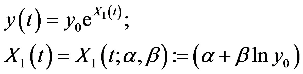
where  is income per capita (GDP) at the beginning of research (t = 0), and
  represents growth rate of GDP at t. For economic thesis that economic growth rate definitely develops, where per capita growth rate negatively depends on primary income and gradually becomes lower and then convergent at stationary state at the end (if these economies have very similar structures), we consider 2 following models from Barro models in [1,2] for growth rate as:
Expanding Barro Model
 (6)
(6)
When considering model 1, we put:
 (7)
(7)
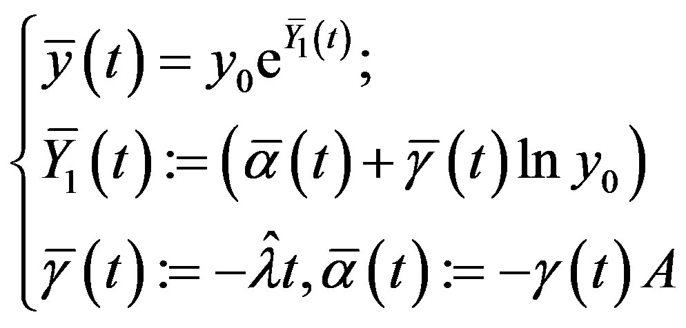
And we get solution for (6) under form:
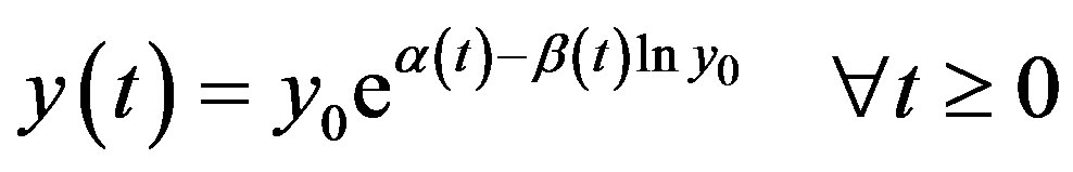 (8)
(8)
Then, it’s easy to see the form of convergence condition for the problem:
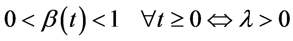 (9)
(9)
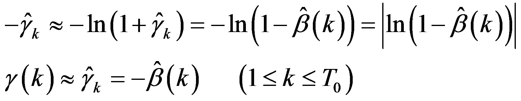
From this condition, we infer:
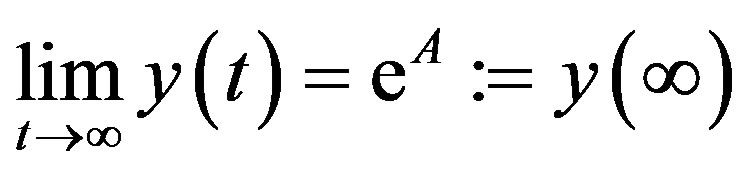 (10)
(10)
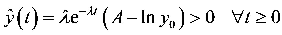
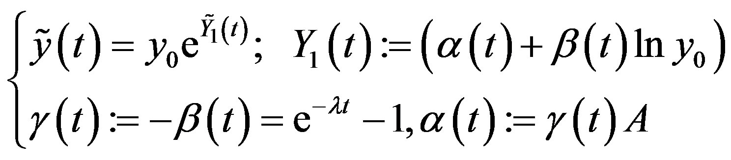
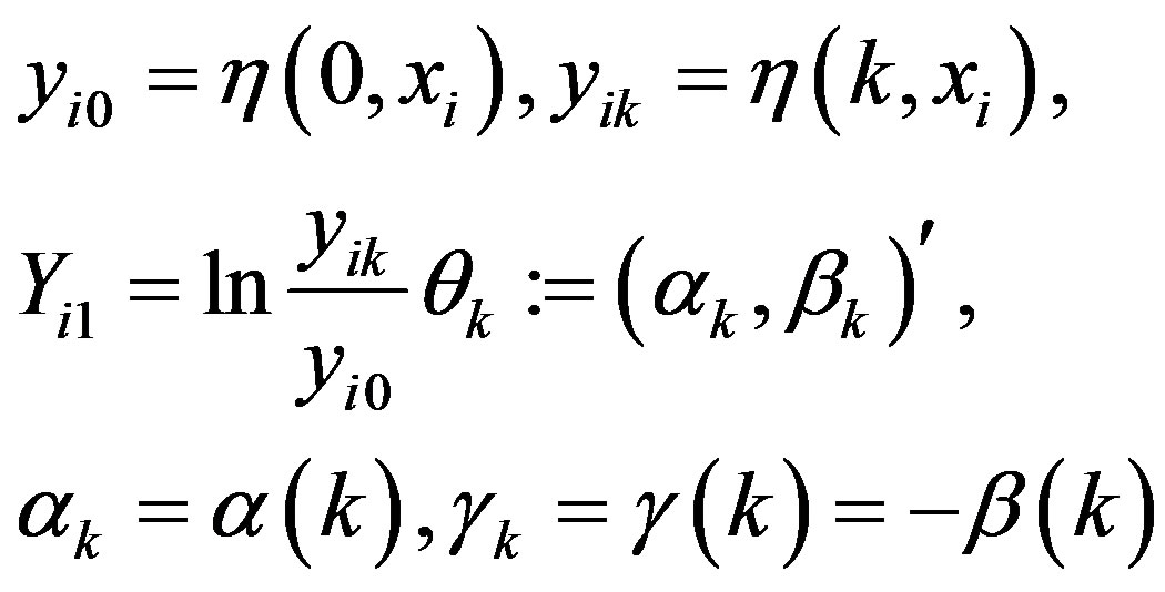
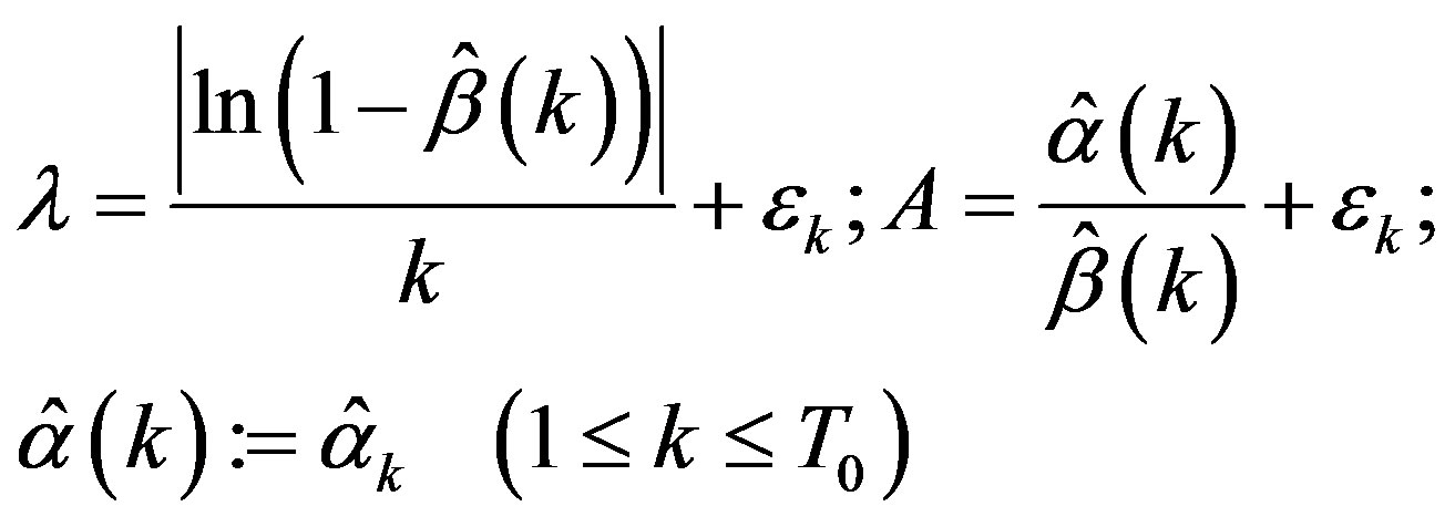
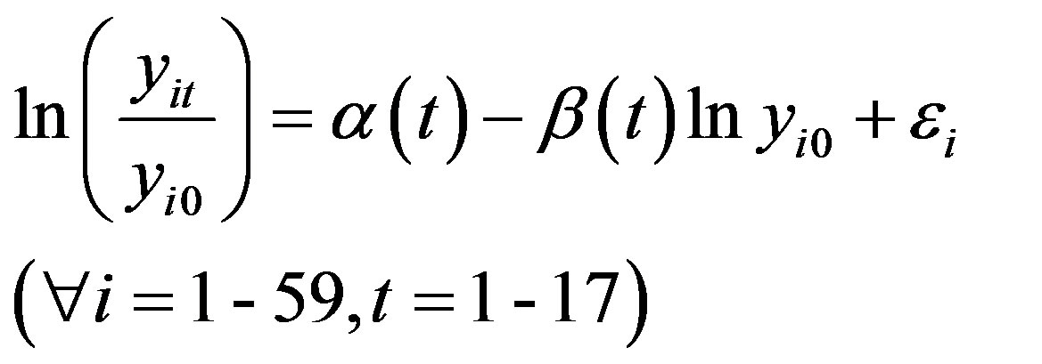
To identify regression model for determine parameters A, λ in the model at studying time (0, T), (8) is taken a logarithm and we obtain:
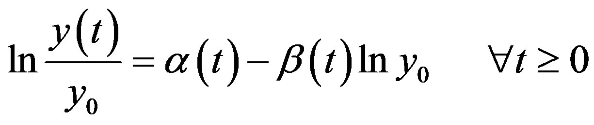 (11)
(11)
And following algorithm.
Algorithm 2.1. (Convergence of Expanding Barro model):
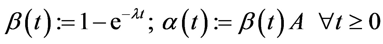
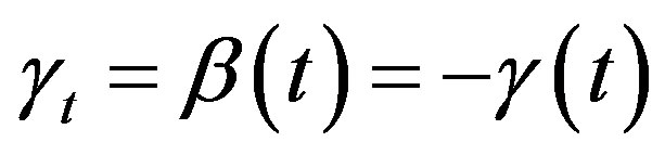
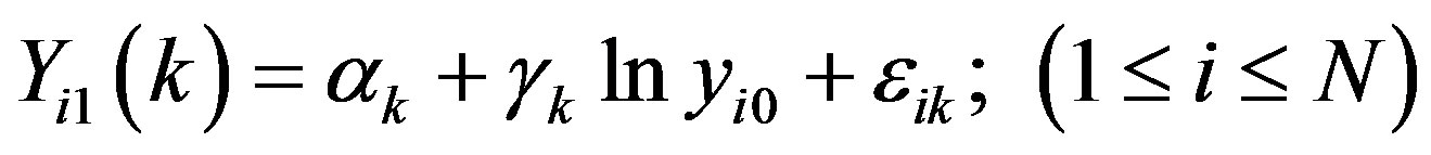
Step 1: For every period (year) t = 1 - T at time study, we set up N linear regression equations in accordance with parameters α(t), β(t) based on (11):
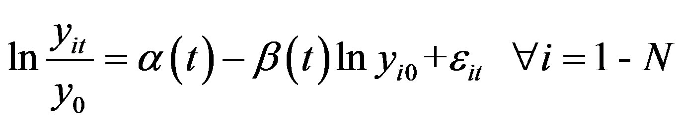 (11a)
(11a)
where  is observable data
  at sub-region (province)
  with respective error .
Let  are least square estimators of parameters
  achieved from above regression model.
Step 2: Apply (9) to check convergence condition :
:
a—if the condition (9) is unsatisfied with every t = 1 - T, problem (1) will be concluded not to be convergent and then stop computing.
b—with all  for instance we next to Step 3 if the condition is satisfied.
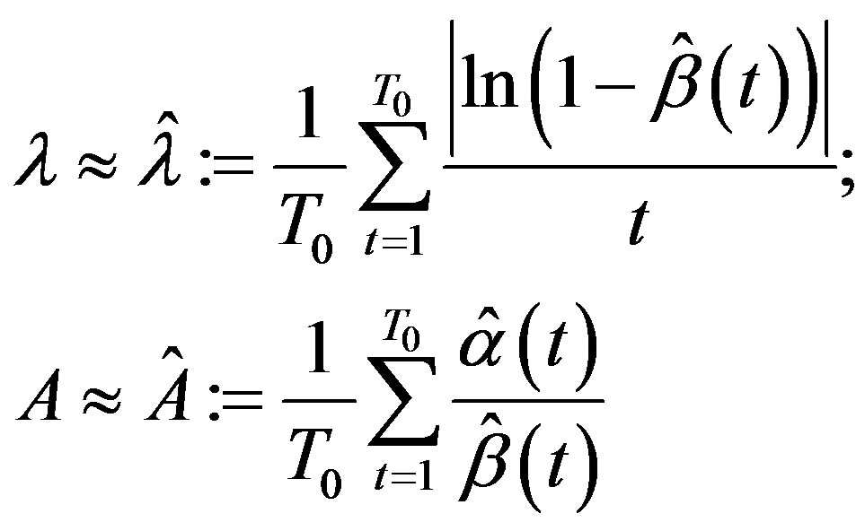
Step 3: We obtain least square estimators for model parameters based on (7):
 (11b)
(11b)
where  represents convergence speed of the economy and from (10), we refer:
 .
.
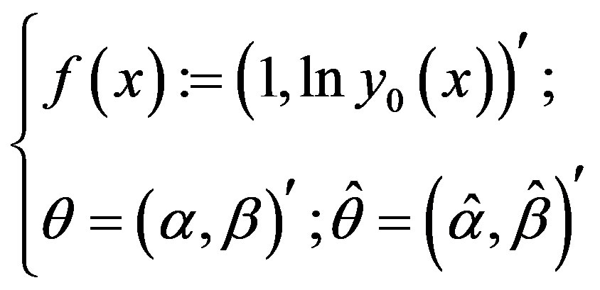
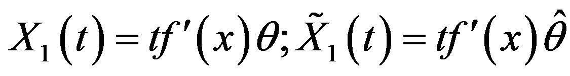
In comparison models in the algorithm with classical Barro model, we initially consider the regression model, and defined parameters α, β in function:
 (12)
(12)
where  with
with  as observable variables; t = T is time control variable;
  represent space control variables (sub-region). Attaching resulting observations, we set:
 (13)
(13)
 (14)
(14)
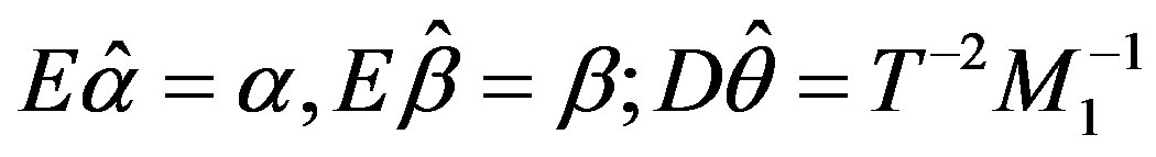
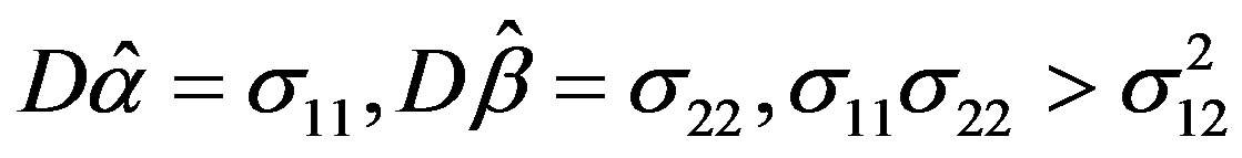
where  are least square estimators of α, β from the system of N regression Equations (4). We then have statement as follow:
Lemma 2.1: If  and denote:
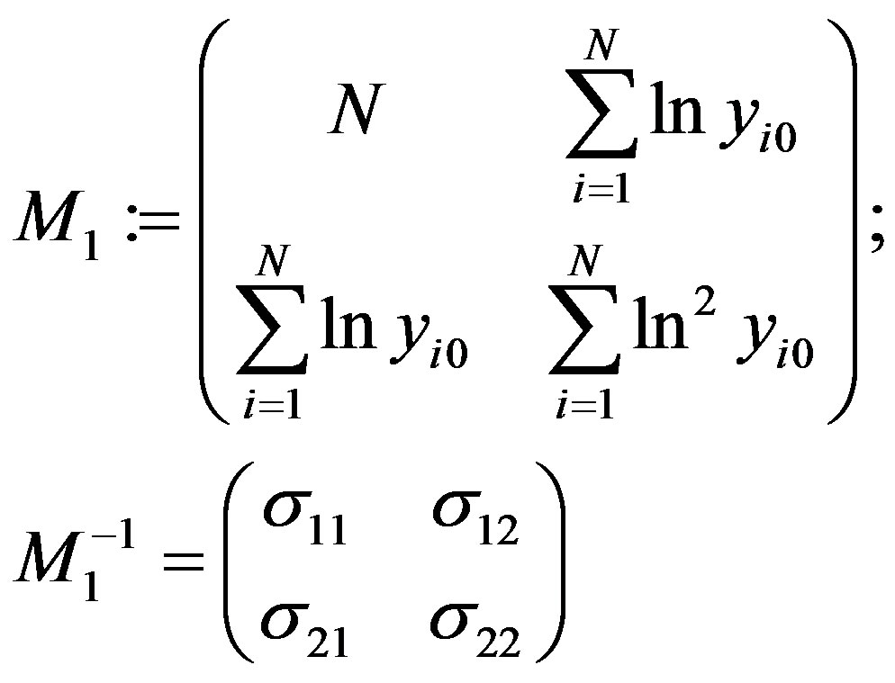 (15)
(15)
With all  we have:
 (16)
(16)
where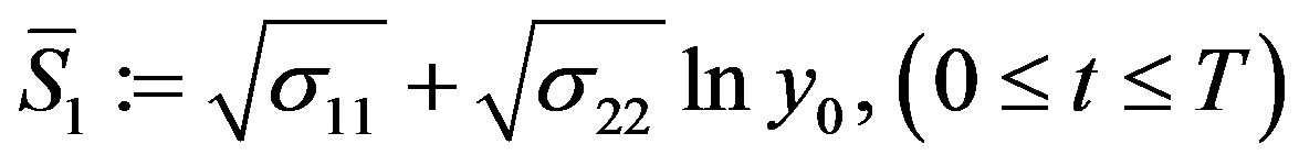 .
.
Proof: When we put
 (17)
(17)
We have (see (12), (14)):
 (18)
(18)
From (14), we also refer classical Barro regression Equation (4) with linear form as:
 .
.
Hence, for least square estimator  of
of , we have (see (15)):
 (19)
(19)
Besides, for symmetric and positive determination of matrix D, we also have:
 .
.
Then, from (18) and (19) we have:
 (20)
(20)
Besides, from (12), (14), (19), we refer:
 .
.
Then, use Chebyshev inequality from (23):
This established the result. ¨
Now, we consider Expanding Barro Model attaching defined parameters λ > 0, A in (10), (11). In this case we have:
 (21)
(21)
where  with
with  as observable parameters; t = T represents time control parameter and
  are space control parameters (at sub-region
 ).
).
For each t = k (1 ≤ k ≤ T) we put:
 (22)
(22)
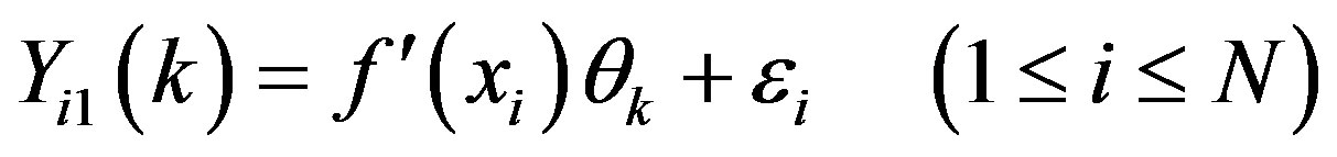
N regression Equation (11a) for specifying 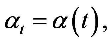
 (t = k) have linear form as:
 (23)
(23)
Let  is least square estimator of parameters
  in (23). Not to loose generality, we suppose:
Let  are respective least square estimators of λ, A in corresponding regression equations:
 (24)
(24)
Put:
 (25)
(25)
And we obtain proposition as:
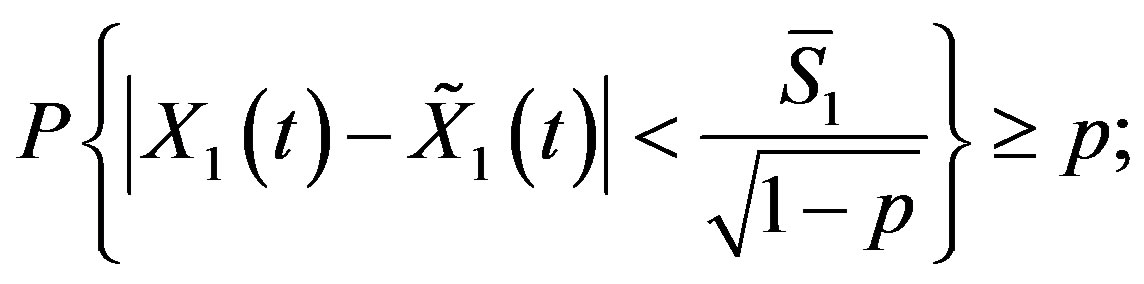
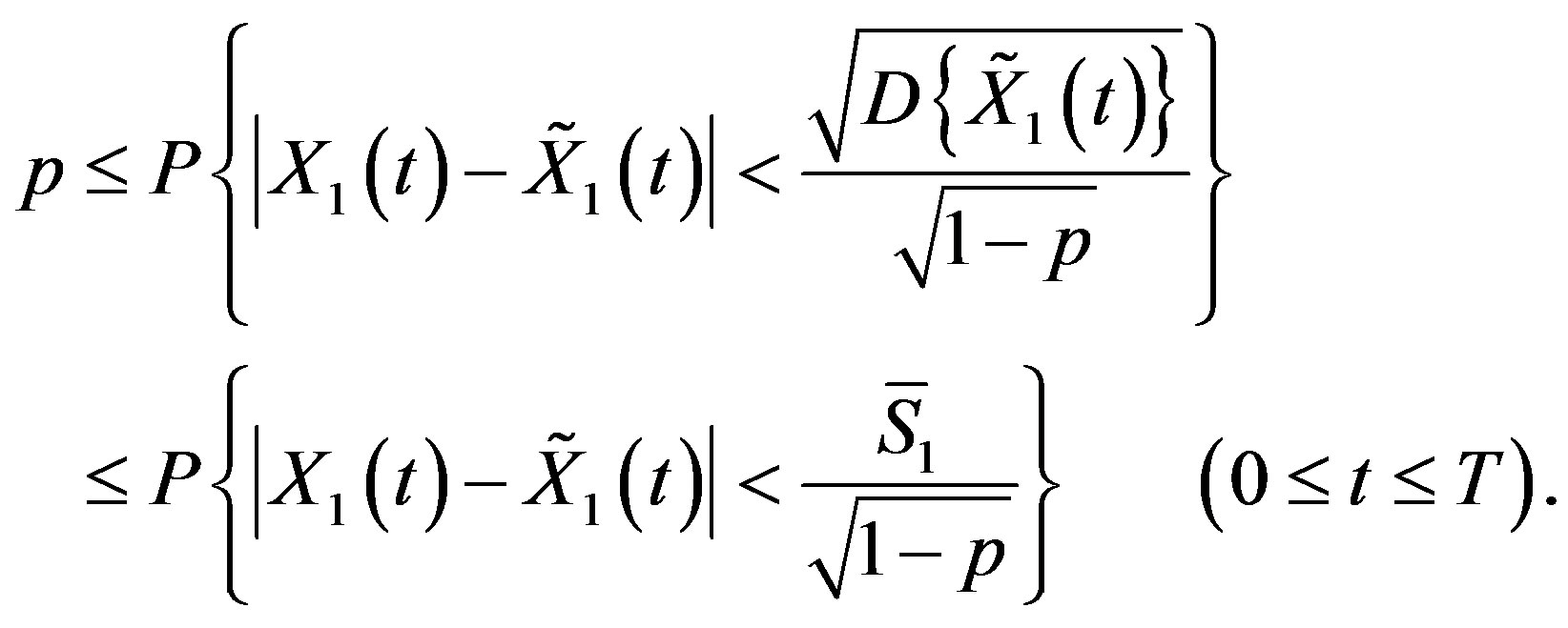
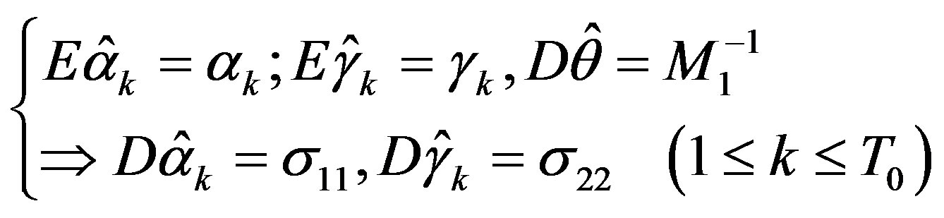
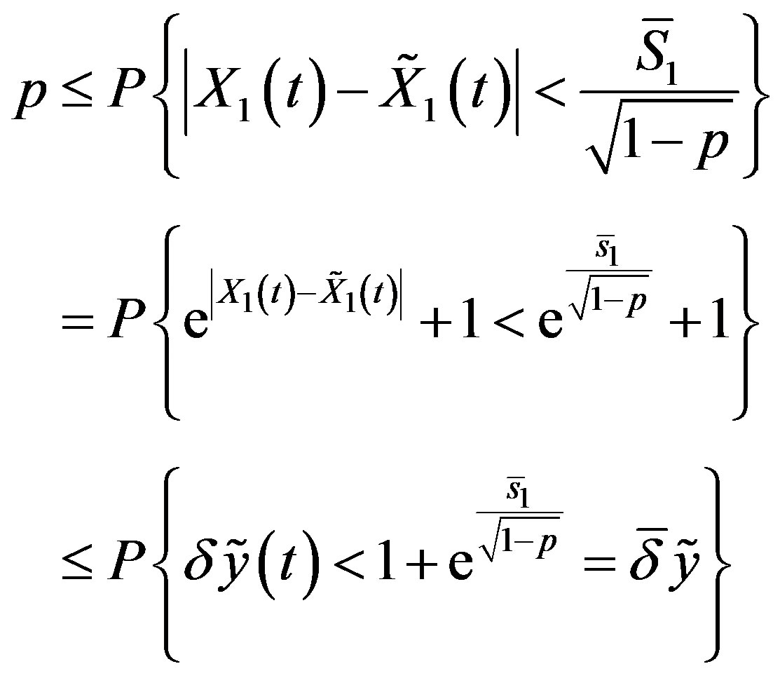
Lemma 2.2. If  and
and  (small enough), we have:
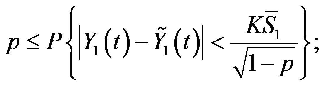 (26)
(26)
where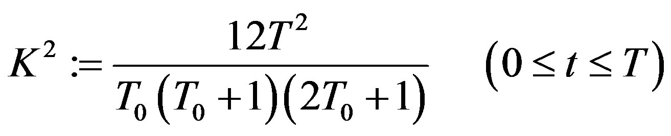 0 < p < 1 and we obtain approximate value of
  for (11b) at
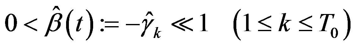
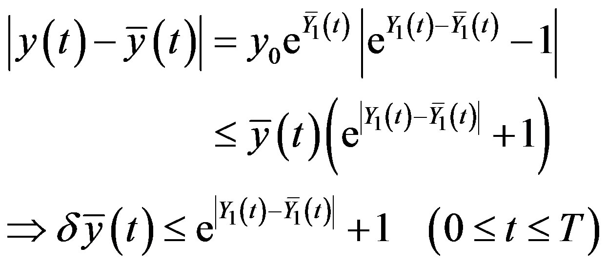
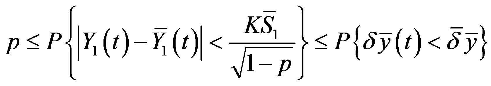
Proof:
For vectors of  in (17), the N regression equations are displayed under form:
On the linear form of parameters , least square estimators
  for parameters
  are likely to be achieved, where (see (15)):
 (27)
(27)
Similarly, for  primary regression equations in (24), as they are under parameter λ-based linear form and observable variable
  includes variance
 least square estimator
  of λ satisfies:
 (28)
(28)
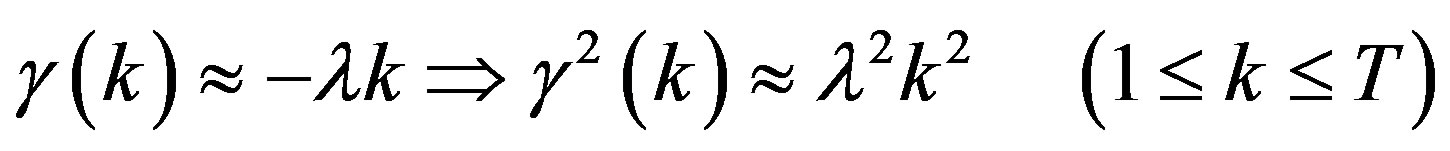
When repeating the above provement for  of the second regression equations in (24), we can see that thanks to observable variable with variance
  (see (27)), we have:
 (29)
(29)
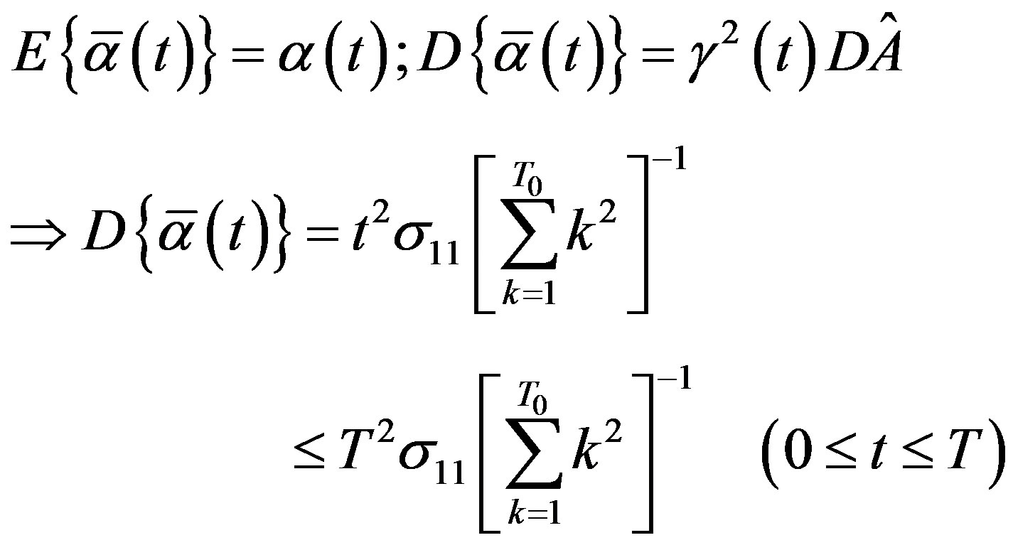
with  is least square estimator of A.
Due to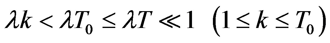 , it can be referred from (21):
Then, from (21), (25), (28), (29), we have
 (30)
(30)
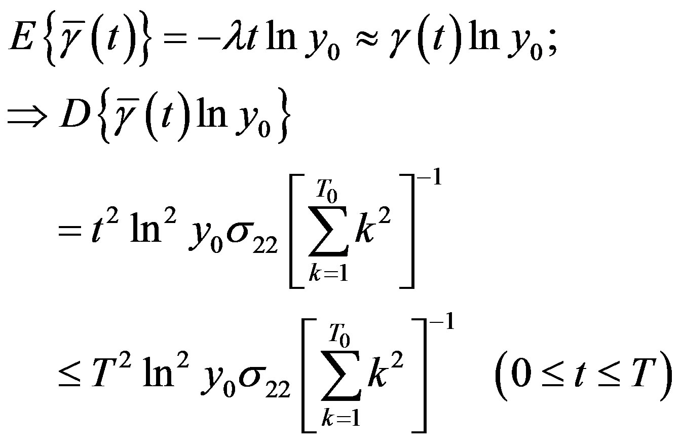 (31)
(31)
From (30) and (31), we can employ inequality Chebyshev to gain:
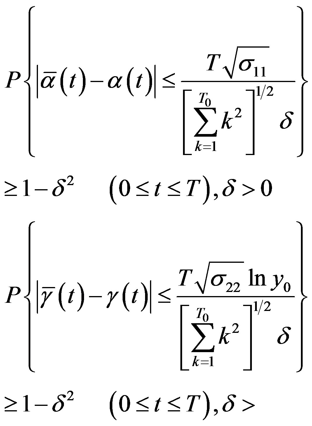
in succession.
At that time:
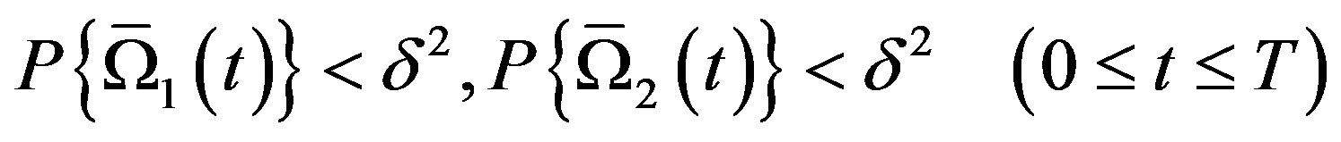
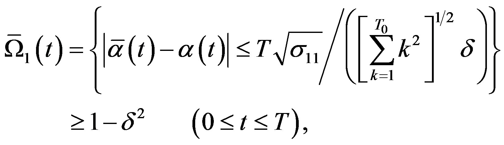
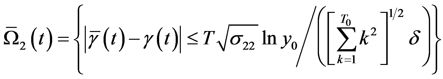
Base on this algorithm and D’Morgan rule, we achieve:
That means (review (21), (25), (26)):
Because  so when setting above formula as
 , we get (26) ¨
When 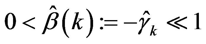 we have:
At that point, recurrent Equation (24) is approximately at:
Therefore, we can evaluate the least square estimators  of
of  in the mentioned recurrent equations by Formula (11b).
Aiming to indicating the preeminent advantage of expanded Barro, we provide following algebraic clause:
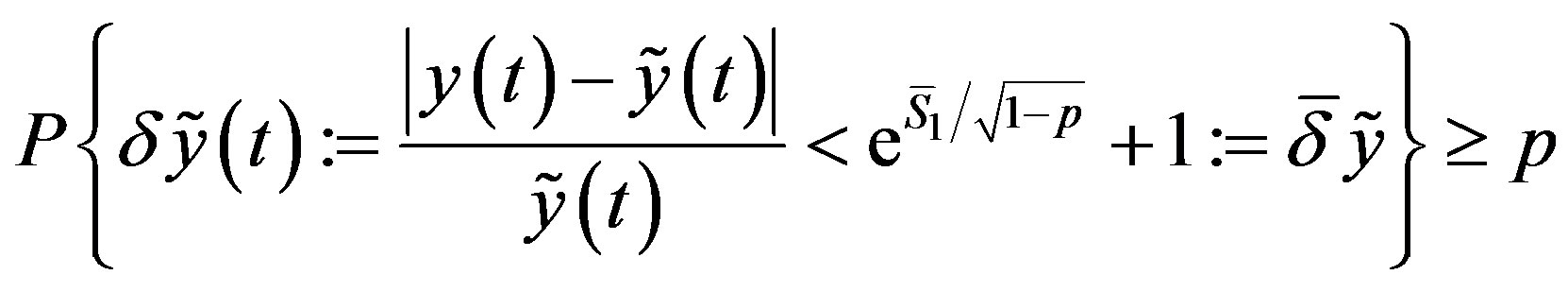
Theorem 2.3. If the conditions of Lemma 2.2 are met and
 (32)
(32)
We can examine the relative error  of the approximate function
  (under classic Barro) and
  (under expaned Barro) by the formulas:
 (33)
(33)
 (34)
(34)
With the reliability p, the estimated value of relative error under classic model sees small disparity compared to its of expanded model:
 (35)
(35)
where
 (36)
(36)
Proof: Firstly, from the value of constant  in (26) and condition (32), (36) can easily found. Besides, (12) (14) infer:
At this point, (16) can lead to:
That means we successfully prove (33).
Similarly, from (21) and (25), we also get
Therefore, we have
from (26) and (34) is demonstrated. Finally, from expression of  (in (33)) and
  (in (34)), we can use
  in (36) to get (35). ¨
The algorithms to evaluate errors (35) and (36) introduced in above theorem aim to compare classic Barro with its expanded one in the period  when they fully meet the conditions in (32) (close evidently). For example, when
 , this condition is satisfied with
  .
.
However, when solving a problem, we need to take some following factors into account.
Note. Because the LS estimated  of parameters
  in linear regression model (26) is steady estimation:
In the same way, for the LS estimated  in recurrent models (24) we have:
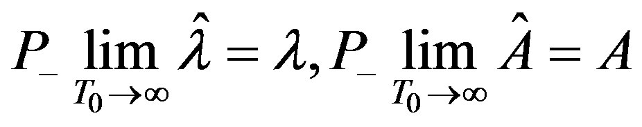
Now, (review (24), (25)):
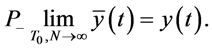
That means  (enough big) leads to
 .
.
2.3. Markov Chain Models
Consider problem (1) with  being a per capita income process,
  is regarded as a/an (stochastic) income per capita process in fact such that
 . Divide the income per capita into n levels
  with
with 
and put  as probability distribution of
  following mentioned earnings level:
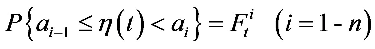
We have
 (37)
(37)
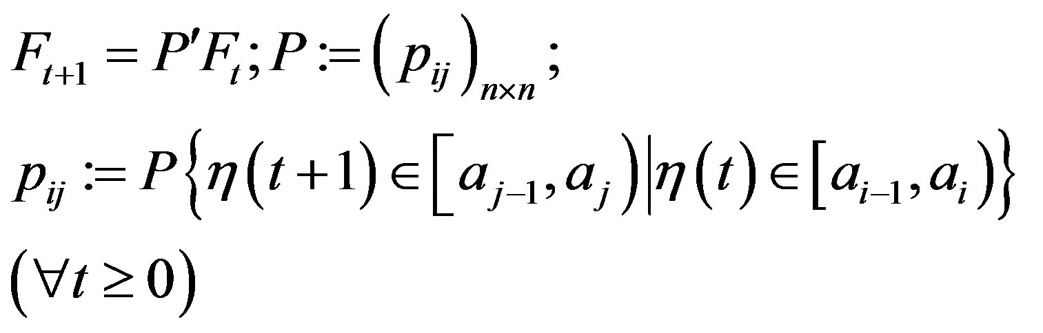
If Markov chains are then homogeneous responding to ergodic transition probability matrix , we have:
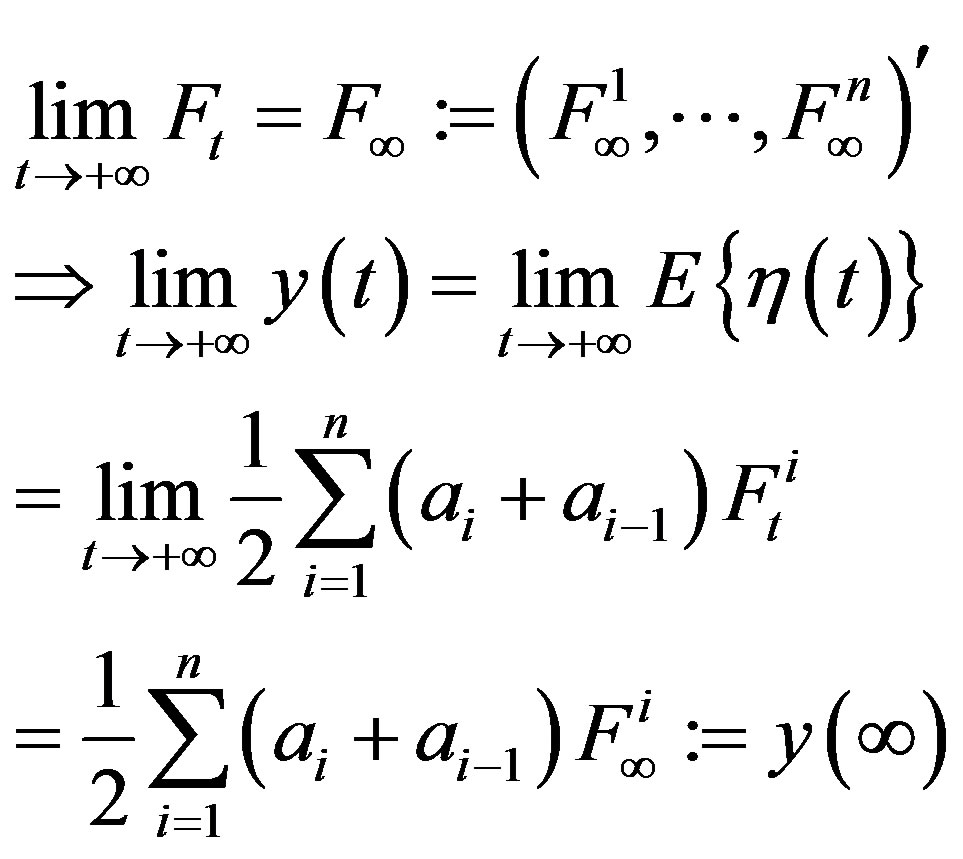 (38)
(38)
This is the reason for us to convert convergent problem (1) research into valuate the homogeneous and ergodic Markov chains. Homogenisation suggests that the probability of some province belongs to  at
at  will fall into
  at
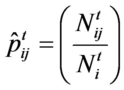
at  as constant over time. A maximum likelihood estimation is given by:
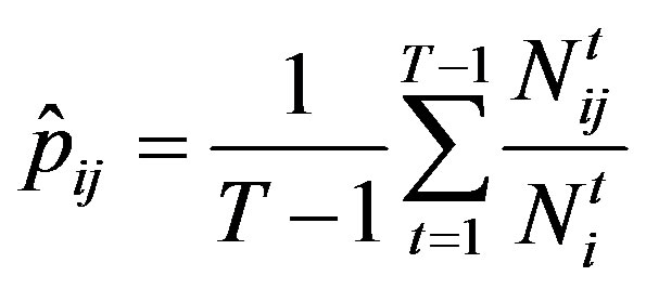
Here,  is the number of provinces transferring from
  to
to  at
at ,
,  is total provinces in
  at
at  and
and  represents processes. To test the invariability of the transition probability over time, we evaluate twin of following hypotheses:
Hypothesis:
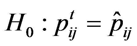
With all  and its assumption as:
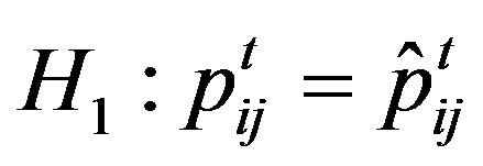
where
is transition probability estimate at . For these hypotheses, likelihood ratio is defined by:
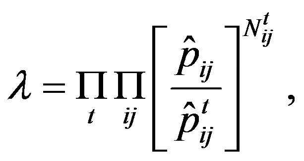
where,  are determined in hypothesis
  and
and  are determined in hypothesis
 .
.
And  is distribution of
  if
if  is true. Therefore,
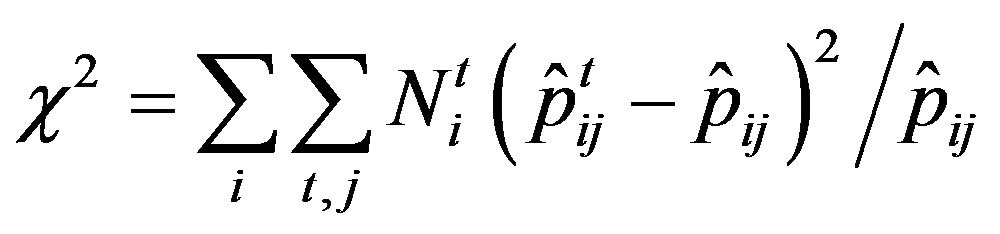
Have distribution if  square is free order. Here,
  is the number of processes,
  is state class of Markov chains.
3. Experimental Estimating Results
Barro Model:
Set independent variables are growing logarithm of per capita income in the province at late , and dependent ones represent income per capita at early stages. After removing inappropriate variables, final estimation for the period of 1990-2007 is as:
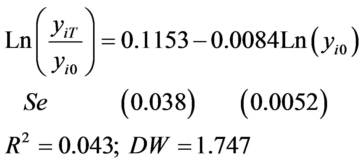
Estimated results shows that negative coefficient β have no  lower significance level
 . We also split into small periods to estimate above equation but no ones see coefficient β statistically better than that of the whole period 1990-2007.
Expanding Barro Model:
From above theoretical models and per capita income data of 59 provinces over Vietnam, we used analysis of regression to analyze the convergence of economic variable GDP (income per capita). For each period (year) , we build 17 regression equations by virtue of cross data:
For these equations, we obtain the estimators for economic convergent speed:
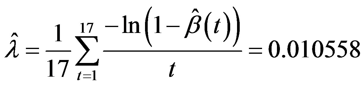
and value
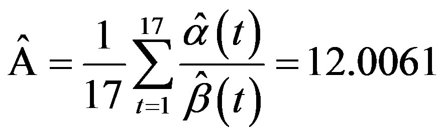
Average earnings at convergent state is
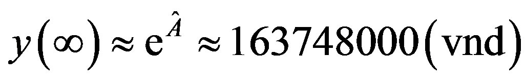 .
.
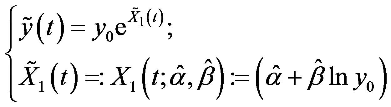
We can use following model to forecast average income in coming years:
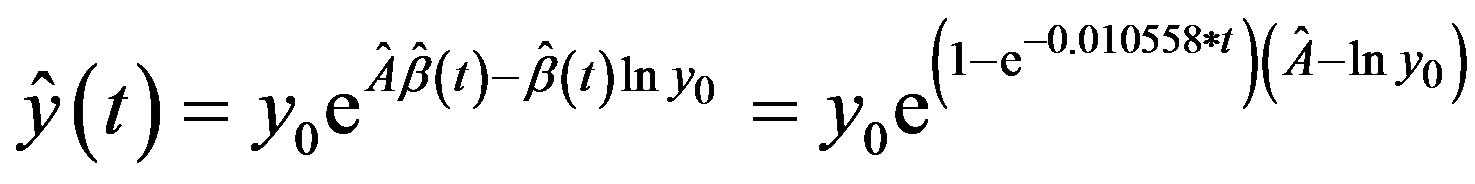 (39)
(39)
We obtain forecasted results as below Table 1.
Here, we denote  is estimator for
 .
.
Markov Chain Model:
Consider parameter  which represents provincial per capita GDP distribution. To disconnect
  under form (12), we use an experimental procedure which
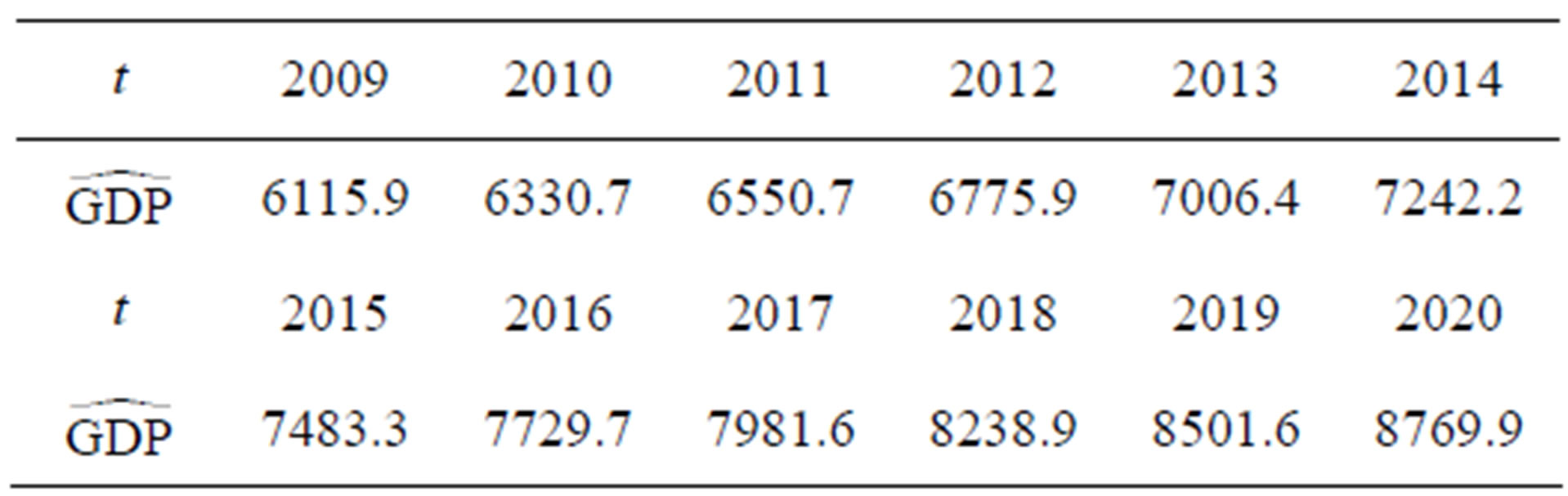
Table 1. Average earnings forecasts (unit: 1000 vnd).
calculates  in the primary period of
  or
or  first, and then sorts them in progressive order. What more, we will divide
  into several intervals so that every interval includes minimum variances. Arranged turning points in
  correspond to thresholds in the intervals, so we have
for gross rate. Experimental results from Markov chains provide deep understanding about changing features of dynamic changing distribution of provincial per capita GDP. mean of  in the periods is considered as an estimator of transition probability matrix P. Distribution
  consists of residual values between provincial average GDP and that of Vietnam.
  is calculated and ranked in order of each process.
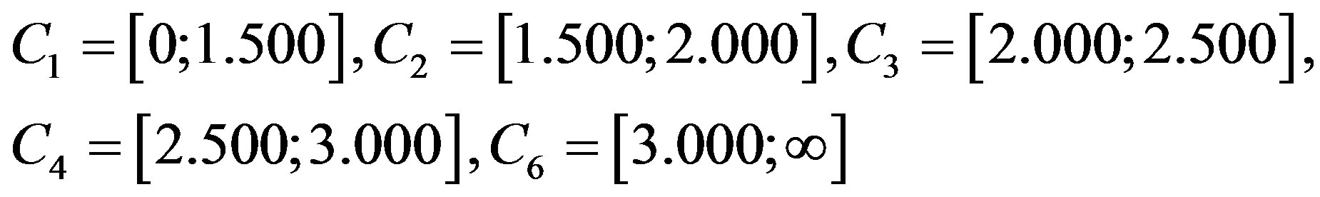
• If a period comprises 3 years, we will have 6*59 observations from 1990 to 2007. The economy will divide into 5 states:
State 1: Average GDP ≤ vnd 1.5 million.
State 2: vnd 1.5 million < Average GDP ≤ vnd 2 million.
State 3: vnd 2 million < Average GDP ≤ vnd 2.5 million.
State 4: vnd 2.5 million < Average GDP ≤ vnd 3 million.
State 5: Average GDP > 3 million.
We have transition matrix system as:
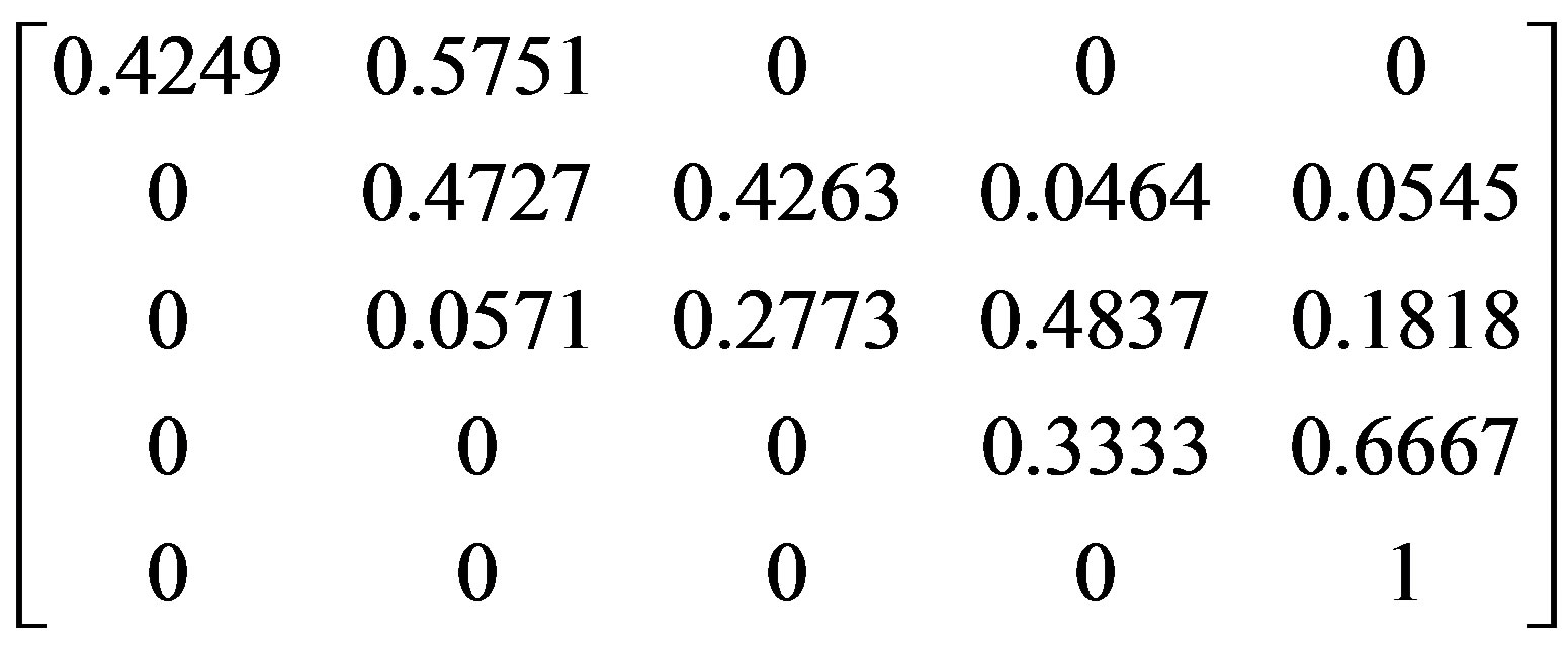
As in this matrix, State 1 provinces with lower VND 1.5 million per capita GDP will consist of  percentage of those who stays at State 1 and
  percentage left comes to State 2 with per capita GDP floating around VND 1.5 - 2.0 million. The remaining does the same. We can see from above matrix that transition probabilities from State 1 to State 2 are greater than State 2 transition probabilities coming to State 3 which remain bigger than State 3 probabilities turning to State 4 after completing a period. This is also convergent sign of the economies.
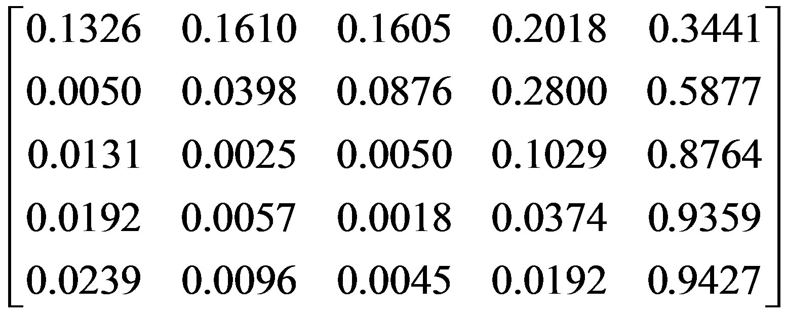
After 5 processes, we have transition probability matrix:
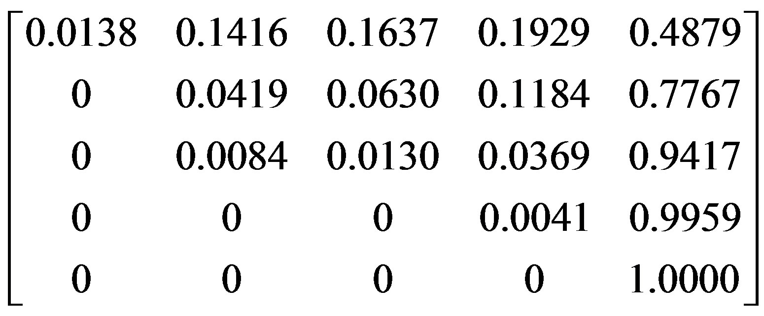
This is the upper triangular matrix with decreasing per capita GDP at States 1 and 2 which indicates convergence mark of the economy. As in this matrix, provinces with high per capita GDP are likely to fall into 0% states after states after 5 development periods. Similarly, 48.79% of province with of province with lower VND 1.5 million per capita GDP ups to higher VND 3 million. We continue to consider convergence at time by far. We obtain following transition probability matrix after 10 periods:
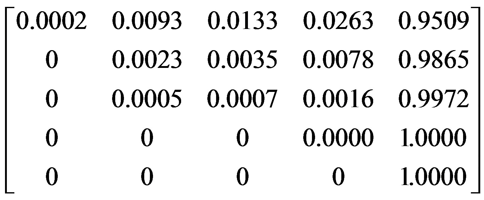
Therefore, 30 years behind remains state 5 called absorbed state. This means that some process falls into state 5 won’t be likely to come to others. Probability distribution during the period of 2005-2007 as:
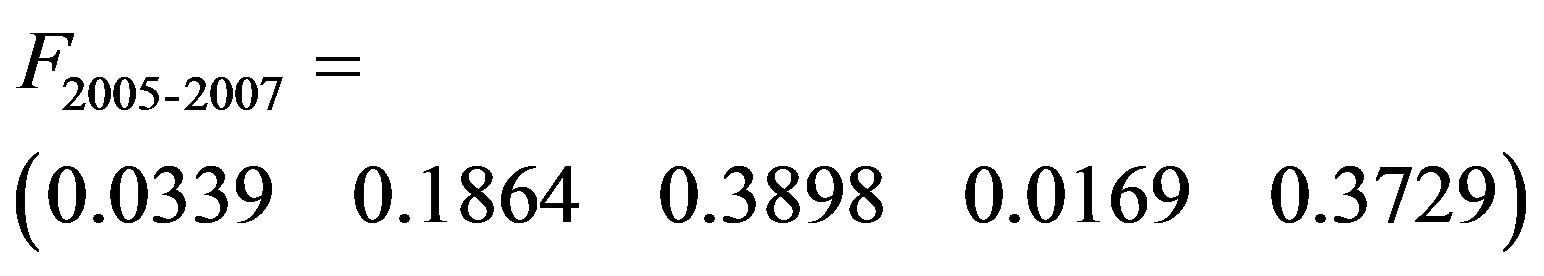
We have probability distribution forecast for period 2008-2010 as:
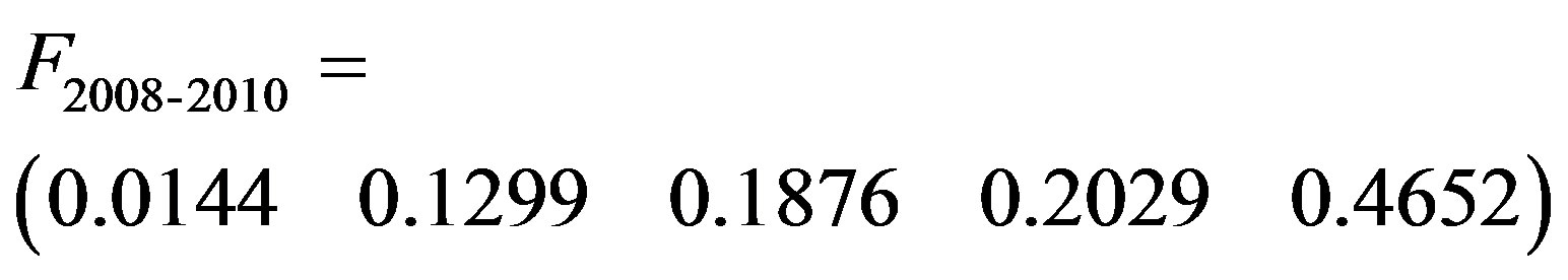
The data indicates  percentage of province with lower VND 1.5 million per capita income,
  fluctuating from VND 1.5 - 2 million,
  with per capita income from VND 2 - 2.5 million,
  remaining income per capita from VND 2.5 to 3 million, and
  with higher VND 3 million per capita income during period 2008-2010.
Consider process consisting of one year from 2003 to 2007, there remains  observations. We just consider lowest state (lower VND 2 million) and highest state (higher VND 3.5 million) for enormous income per capita during this period. We cut our economy in 5 following states:
State 1: Per capita GDP ≤ VND 2 million.
State 2: VND 2 million ˂ per capita GDP ≤ VND 2.5 million.
State 3: VND 2.5 million ˂ per capita GDP ≤ VND 3 million.
State 4: VND 3 million < per capita GDP ≤ VND 3.5 million.
State 5: Per capita GDP ˃ VND 3.5 million.
We obtain transition probability matrix as:
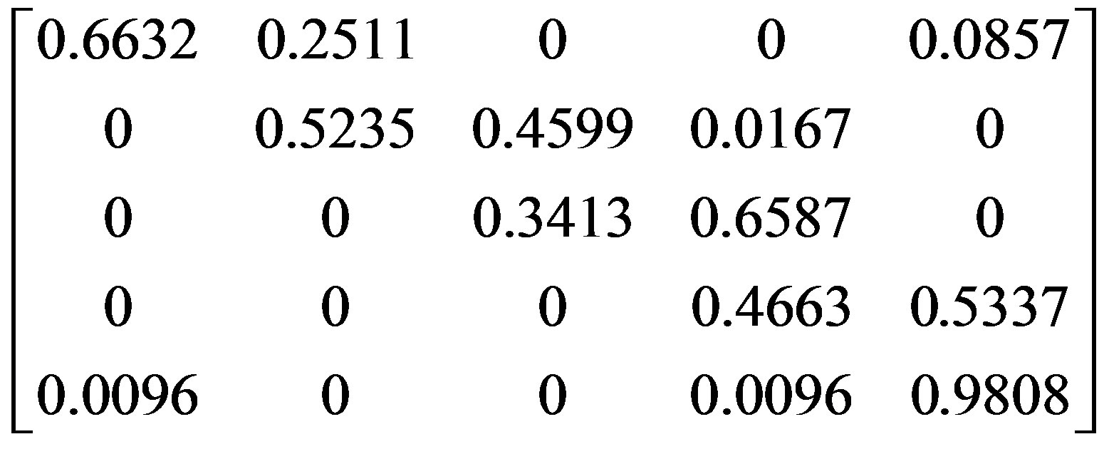
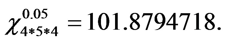
Statistics Chi-square for testing the invariance of probability matrix over time is:
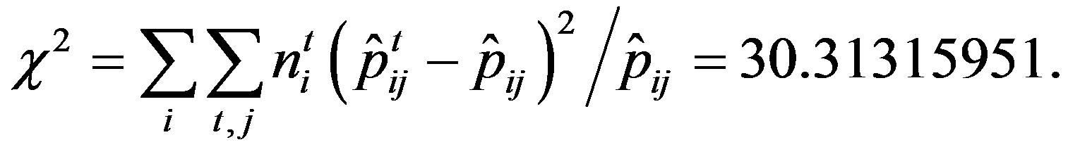
Statistics
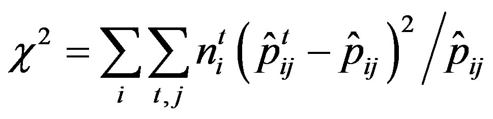
has distribution Chi-square with free order
 .
.
Here,  is the number of periods, and
  serves as the number of state layers in Markov chains. Limitation probability with significance level
  is:
is:
Therefore, we can affirm tested transition probability matrix and use it for forecasting and researching considered ergodic Markov process. In this case, Markov chain is ergodic because all positive elements belong to transition probability matrix level 5
And limitation transition probability represents a transition matrix behind 28 or 30 steps. We have transition probability matrix after 30 years as:
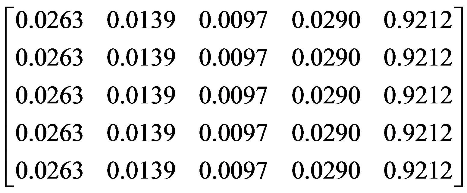
Based on this result, State 5 is living but others are nearly gone out. Yet, State 1 remains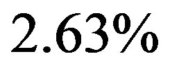 . Hence, we have distribution forecast for 2008, 2009, 2010 and 2020 as follow:
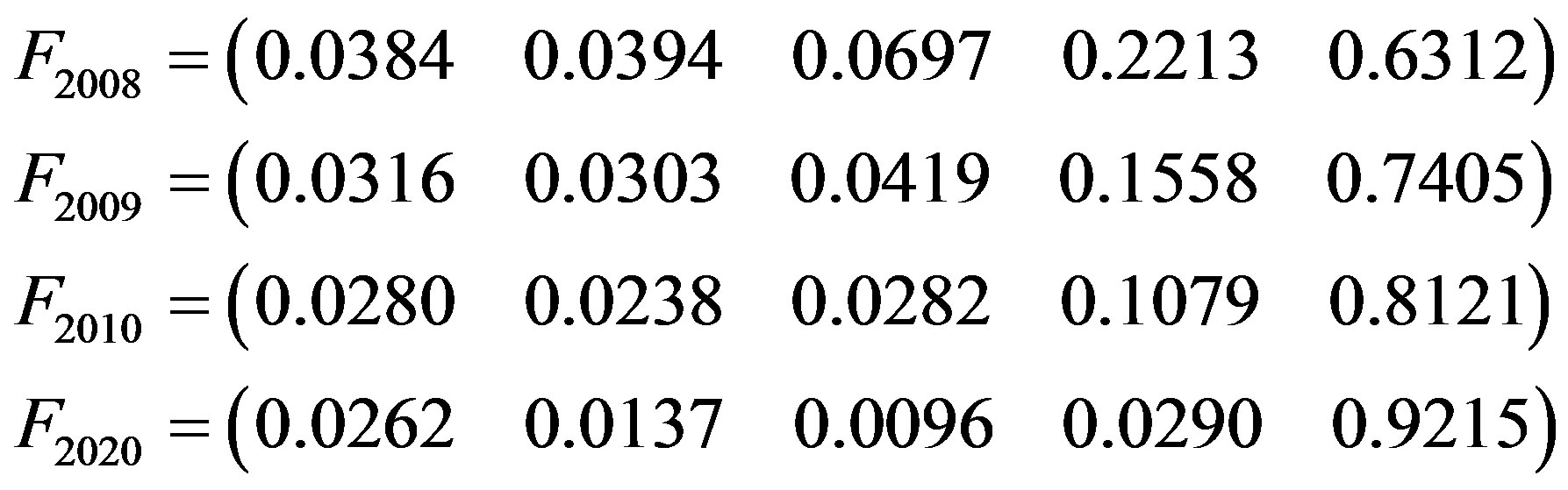
Estimated results show that although there are signs of convergence, this process takes place in a very long future, about 30 years more. Predicted average value in 2009 was approximately calculated as follows:
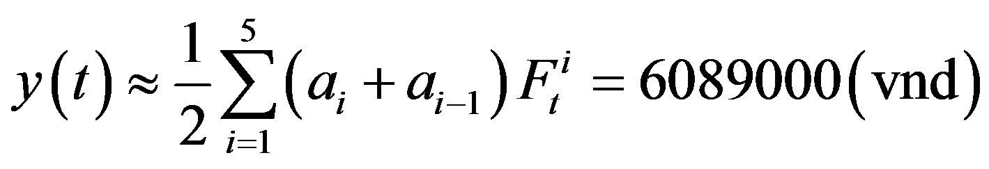
In 2010, it is 6397000 (vnd) and it will be 8701000 (vnd) in 2020.
4. Comparison to Classic Barro Models
Attaching the same data set N = 59, T = 17 of Vietnam’s provinces within 1991-2997, we found that the results calculated under the algorithm 2.1 share the general point with Markov chain algorithm in the fact that the results indicate the common characteristic, the convergence of the model (1).
However, if using classic Barro models for the same data set, we have not yet found common characteristics mentioned above. This is also explained by theorem 2.3 related to the lack of accuracy in classic Barro models compared to corresponding extended models.
5. Conclusions
This research has used different methods to study the income convergence of Vietnam’s provinces within 1990-2007. The estimation results from Barro regression models show that Barro model (1) doesn’t have statistic meaning. Estimated results from expansion Barro regression models based on cross data indicate signs of convergence over the whole study period. Results from extended Barro model are consistent with the results under approaching method based on Markov chains and it has been proved that the error from extended models is smaller than from classic Barro models.
With current situation and no change in policy and regime, according to expanding Barro model, Vietnam’s income per capita is about 8000 USD/year which is very low compared to the developed economies today. Markov chain model is used to illustrate long-term fluctuations within average growth in income per capita among 59 provinces across Vietnam in 1990-2007. Estimation result from Markov chain model indicates convergence signs in distribution but it should be in over 3 decades’ time. The reason might be obstacles in regime which slows down technology transition process leading to limited mobility. Moreover, lack of necessary infrastructure and unfair distribution causes technology diffusion slowdown. The speed of this process may vary among provinces.
6. Acknowledgements
This research is funded by Vietnam National Foundation for Science and Technology Development (NAFOSTED) under grant number II 2.2-2012-18.