Confounding of Three Binary-Variable Counterfactual Model with DAG ()
1. Introduction
Causal inference has become an important research field in statistics, data mining, epidemiology and machine learning etc. in recent decades [1-7], and directed acyclic graph (DAG) is involved in describing the relationship between causal connections [4]. Confounding and confounder are two basic concepts for epidemiology causal inference [1,3]. Several models have been presented for causal inference, two of which are the causal diagram model and counterfactual model [6,8,9].
To assess confounding and confounder, two main approaches, “collapsibility-based” and “comparability-based”, are discussed in [10], which regard confounding bias as arising from differences between stratified measures of association and the corresponding original measure or from the exposed and unexposed populations which are not comparable. The comparability-based approach determines a factor to be a confounder if adjusting for it can reduce confounding bias [3,10]. Geng et al. (2002) [11] point out that the effect of exposure on the rate of a disease cannot be assessed correctly in the presence of confounding bias. They propose probability criteria for confounding and discuss confounding with multi-value covariate variables. However, their work does not clearly analyze general causal DAG even with three binaryvariables, since the simple case of their definition about covariate can only be expressed by Figure 1 (see Figure 6.2 in p. 61, [12]).
As to three binary-variable DAGs, [5,13] discussed identifiability of the causal effect of the other two kinds of counterfactual models (Figures 2 and 3) using the independence hypotheses respectively. Yet, the confounding and confounder in these two simple causal DAGs are not discussed explicitly. For Figure 2 (see Figure 6.5 in p. 64, [12]), the covariate C is an intermediate variable in the causal chain. [6,12] (p. 30) discuss the intermediate variable causal chain, however more variables are involved
in fitting “Back-door” formula and “Front-door” formula.
Traditionally, a confounding variable (the precise definition of a confounder) is a variable which is a common cause of both the control variable and the response variable [14] (see Figure 1). Whether the covariate variable, which is not a common cause of both the control variable and the response variable in three binary-variable counterfactual models, is a confounder? [1,10] develop a qualitative definition of confounder: controlling a variable can reduce confounding, then the variable is called a confounder. Hence, the covariate variable, which is not a common cause of both the control variable and the response variable, but affects the response variable, may be a confounder. Recently, the confounder and confounding detection attracts more attention in gene network discovery [15], the question arises from how to investigate the causal DAG in a pure gene network and how to analyze the role of covariate from statistical data if we think that there is causation structure in gene network? It is necessary to discuss the confounder and confounding in the general causal DAG diagram. These motivations drive us to investigate the confounding and confounder in general causal DAG with the definitions in [11].
In this paper, according to the precise definition, one model as shown in Figure 1 is discussed: the covariate variable affects the control variable and the response variable at the same time, and the control variable affects the response variable. By the qualitative definition, we investigate other two models: one, as shown in Figure 2, is that the control variable has the effect on the covariate variable and the covariate variable affects the response variable; the other, as shown in Figure 3, is that the control variable is independent to the covariate variable and the covariate variable affects the response variable. Obviously, the third model is the special case of the other two models with independence of the control variable and the covariate variable. Then we use the formal definitions of a confounder and an irrelevant factor in [11] and the ancillary information based on conditional independence hypotheses [5,13] to discuss the confounding of above-mentioned counterfactual models.
The rest of the paper is organized as follows: In Section 2, we introduce the main notation and definitions, and discuss the relationship between confounder and irrelevant factor. In Section 3, confounding and irrelevant factor of three kinds of three binary-variable counterfactual models with DAGs are discussed respectively. The conclusion is given in Section 4.
2. Notation and Definitions
Let E, D, C be binary variables. Let the control variable E be an exposure with the values  and
and  representing “exposed” and “unexposed” respectively. Let the response variable
  be an outcome with the values 0 and 1 denoting the presence or absence of a disease, where
  is the corresponding response when
  and
and  is the corresponding response when
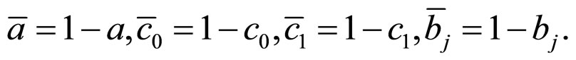
 , both of which take values 1 or 0 denoting the presence or absence of a disease. Let
  be a covariate variable with possible values 0 or 1.
Many kinds of studies focus on the effects of exposure on the rate of a disease in the exposed population. Let  and
and  be the proportions of diseased individuals in the unexposed population and the exposed population. Let
  be the hypothetical proportion of individuals in the exposed population who would have attacked by the disease even if they had not been exposed. Since
  is a hypothetical proportion, the model is a counterfactual model [8,9].
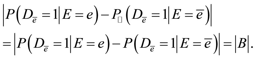
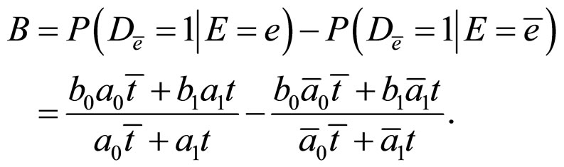
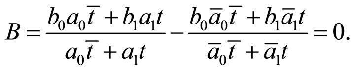
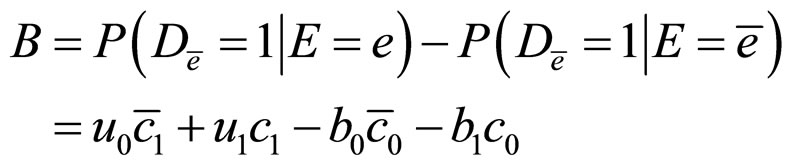
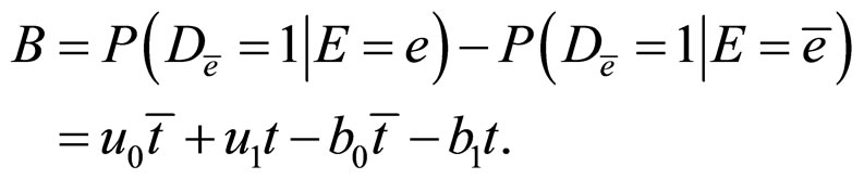
In order to identify the casual effect of exposure on response, confounding bias  is defined as the difference between the hypothetical proportion of diseased individuals in the exposed population [16,17], that is
 (2.1)
(2.1)
If , then there is no confounding.
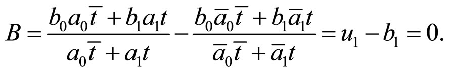
By the common standardization in epidemiology [1,2, 11,18-20], the standardized proportion , which is obtained by adjusting the distribution of
  in the unexposed population to that in the exposed population, is
 (2.2)
(2.2)
Definition 1 [11]. A covariate  is a confounder if
 (2.3)
(2.3)
From the definition, we find that the standardized proportion  obtained by adjusting for the irrelevant factor is closer to the hypothetical proportion
  than the observed proportion
 .
.
Definition 2 [11]. A covariate  is an irrelevant factor if
 (2.4)
(2.4)
Since the estimation of the hypothetical proportion is still unchanged after being adjusted for an irrelevant factor, we do not need to adjust it to reduce confounding bias. And, the relationship between irrelevant factor and confounder is obtained in Lemma 1:
Lemma 1. If a covariate  is an irrelevant factor, it is not a confounder. Inversely, if
  is a confounder, it is not an irrelevant factor.
Proof.
According to the condition that  is an irrelevant factor, we can obtain that
Then,
which means  is not a confounder.
From the condition that  is a confounder, we can obtain
Then,

In fact, if
 Then,
Then,
This is a contradiction!
Hence,  is not an irrelevant factor. □
[11] (pp. 7-8) gives an example, and illustrates two cases of irrelevant factor and confounder respectively. To illuminate conceptions of confounding and irrelevant factor and Lemma 1, we continue to discuss the relationship based on their original example and give two examples as follows.
Example 1. For example in [11]. Let a factor  express groups categorized by every 10 years of age, and its values 1, 2, 3 and 4 denote the original age groups 20 - 29, 30 - 39, 40 - 49 and 50 - 59 years respectively, we denote it as
 . Suppose that there is no exposure effect, i.e. there are only individuals of type 1 (individual ’doomed’) and type 4 (individual immune to disease), and that the joint distribution of disease, exposure and a factor
  is given in Table 1 of [11] (p. 7), where

When the individuals are regrouped by “younger than 50”, we denote it as , which means we adjust the distribution of C, a coarse subpopulation is given in Table 1.
Then,

And,
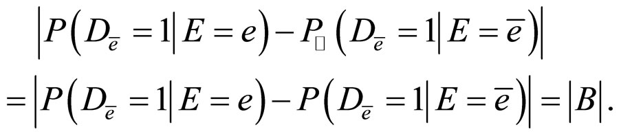
That is,  is not a confounder, and it is not an irrelevant factor.
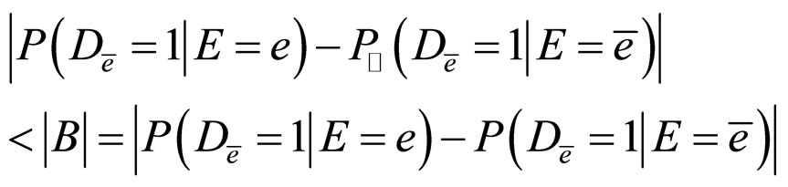
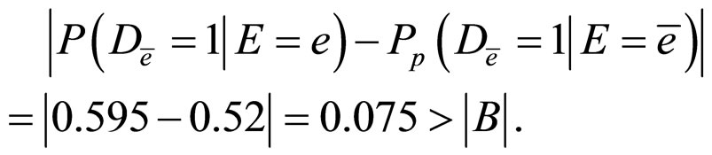
Example 2. To continue the discussion of above example in [11], when the individuals are regrouped by “younger than 40 but older than 30”, we denote it as , we can obtain a coarse subpopulation given in Table 2.
Then,
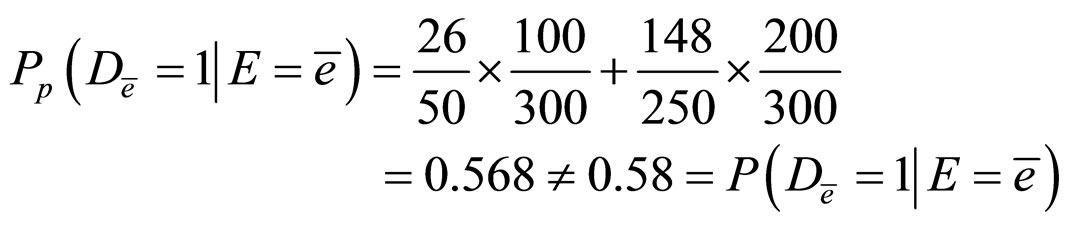
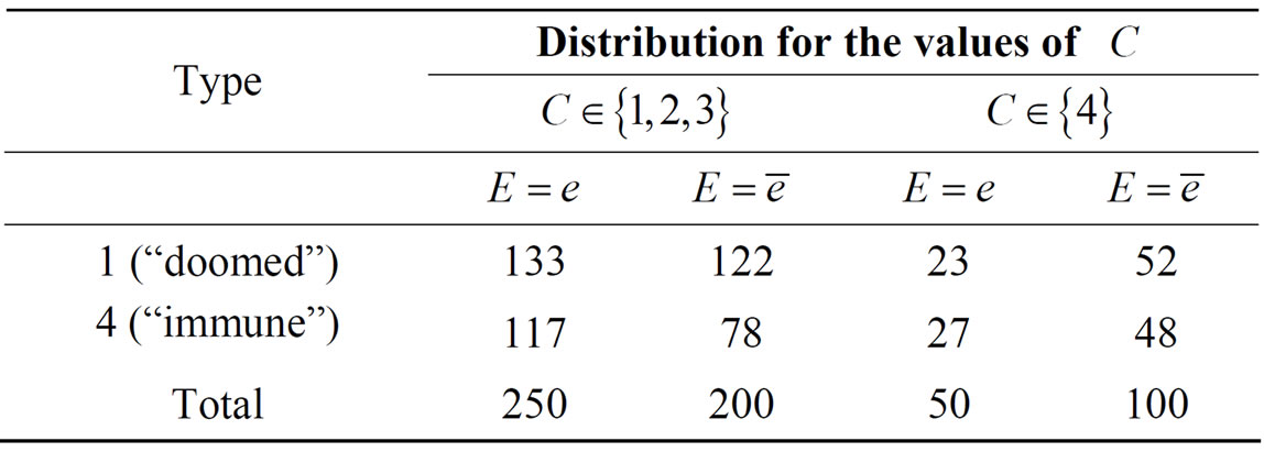
Table 1. Example of a factor C which is neither a confounder, nor an irrelevant factor.
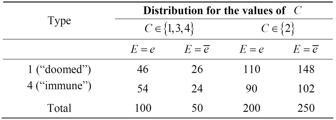
Table 2. Example of a factor C which is not an irrelevant factor, but is a confounder.
Hence,

To sum up,  is not an irrelevant factor, but is a confounder.
As announced in [11], regrouping ,
,  is a confounder, but not an irrelevant factor. Example 2 shows that confounder is not unique,
  is another case, and they have different values of
 .
.
Conclusion: According to Lemma 1, Example 1, Example 2 and [11], whether a factor  is a confounder or an irrelevant factor depends on the adjusting distribution of
 . That is, even for a fixed factor
  in a specific experiment, for example, age, how to judge it as a confounder or an irrelevant factor relies on the “right” adjustment of its distribution. And, more important, the non-uniqueness of confounder makes the causal analysis be more complex.
If we transform the adjustment of covariate variable in Figure 1 to the intervention distribution in counterfactual models in Figures 2 and 3, the definition 1 and definition 2 would be easily employed in the discussion of confounding and irrelevant factor in the other general causal DAGs.
3. Confounding of Counterfactual Model
Considering the confounding of three binary-variable counterfactual models, there are three counterfactual models of causal DAGs as follows (Figures 1-3):
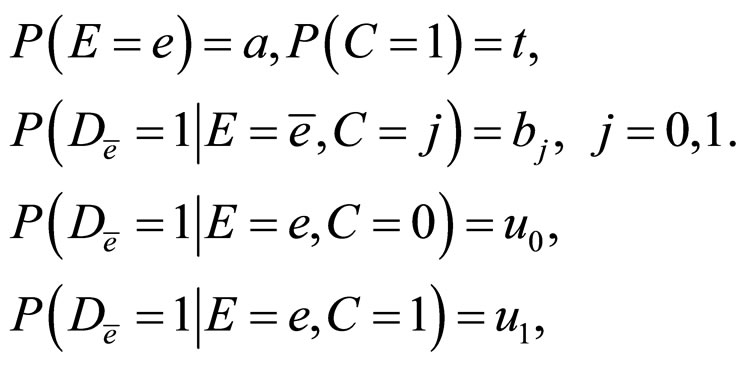
To discuss whether there be confounding in our considering models, we use the conditional independence hypotheses as follows as the ancillary information (H):
1) 
2) 
3) 
4) 
5) 
6) 
7) 
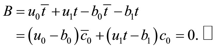
3.1. The First Model
As shown in Figure 1,  has effect on
  and
and  at the same time, and
  affects
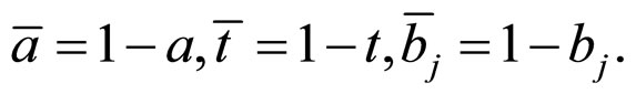
 . In order to calculate simply, suppose that

where  can be observed from original data, but
  can not be observed because they are hypothetical proportions.
Then, we obtain the following formulae,

And,
Using the above formulae, we translate each condition of ( ) into parameter form:
1) 
2) 
3) 
4) 
5) 
6) 
7) 
Theorem 1. If one of the following conditions holds
a) 
b) 
c) 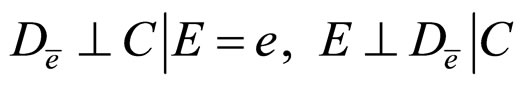
The covariate  is an irrelevant factor.
Proof.
In order to prove  is an irrelevant factor, we only need to prove
That is,
a) From the condition , we can obtain

Then,

b) From the condition , we can obtain

Then,

c) From the condition , we can obtain
 i.e.
i.e. ,
,
 i.e.
i.e. .
.
Since,
We obtain,

Hence,
 □
□
Theorem 2. If one of the following conditions holds
a) 
b) 
c) 
d) 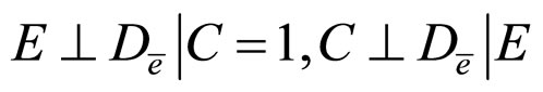
e) 
There is no confounding.
Proof.
a) From the condition , we can obtain

Then,
b) From the condition , we can obtain
 i.e.
i.e. .
.
 i.e.
i.e. 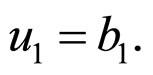
Furthermore,
 i.e.
i.e. .
.
We obtain,

c) From the condition , we can obtain
 i.e.
i.e. ;
;
 i.e.
i.e. 
From the other condition, we obtain
 i.e.
i.e.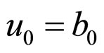 .
.
Then,

d) From the condition , we can obtain
 i.e.
i.e.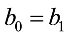 ,
,
 i.e.
i.e. .
.
Furthermore, according to the next condition, we have
 i.e.
i.e. .
.
Then,
e) From the condition , we can obtain
 i.e.
i.e. ;
;
 i.e.
i.e. 
Furthermore,

Then,
 □
□
3.2. The Second Model
As shown in Figure 2,  and
and  have effect on
  at the same time, and
  affects
 . In order to calculate simply, suppose:

where  can be observed from original data. But
 ,
,  ,
,  ,
,  can not be observed because they are hypothetical proportions, also can be treated as counterfactual model by intervention [13].
Then, we obtain the following formulae,


Then,
Using the above formulae, we translate each condition of (H) into parameter form:
1) 
2) 
3) 
4)  i.e.
i.e. 
5)  i.e.
i.e. 
6)  i.e.
i.e. 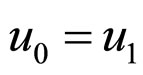
7)  i.e.
i.e. 
Theorem 3. If one of the following conditions holds
a) 
b) 
c) 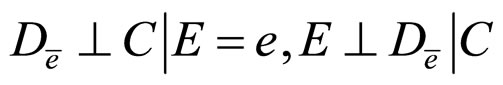
The covariate  is an irrelevant factor.
Proof.
a) From the condition , we can obtain
Then,
b) From the condition , we can obtain
Then,

c) From the condition , we can obtain
 i.e.
i.e. ,
,
 i.e.
i.e. 
Furthermore,
 i.e.
i.e. 
Then,
 □
□
Theorem 4. If one of the following condition holds
a) 
b) 
c) 
d) 
There is no confounding.
Proof.
a) From the condition that , we can obtain
Then,

b) From the condition , we can obtain
 i.e.
i.e. ,
,
 i.e.
i.e. .
.
Furthermore,
 i.e.
i.e. .
.
Then,

c) From the condition , we can obtain
 i.e.
i.e. 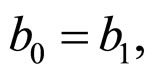
 i.e.
i.e. .
.
Furthermore,
 i.e.
i.e. .
.
Then,

d) From the condition , we can obtain
 i.e.
i.e. ,
,
 i.e.
i.e. .
.
Furthermore,
 i.e.
i.e. .
.
Then,
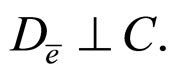
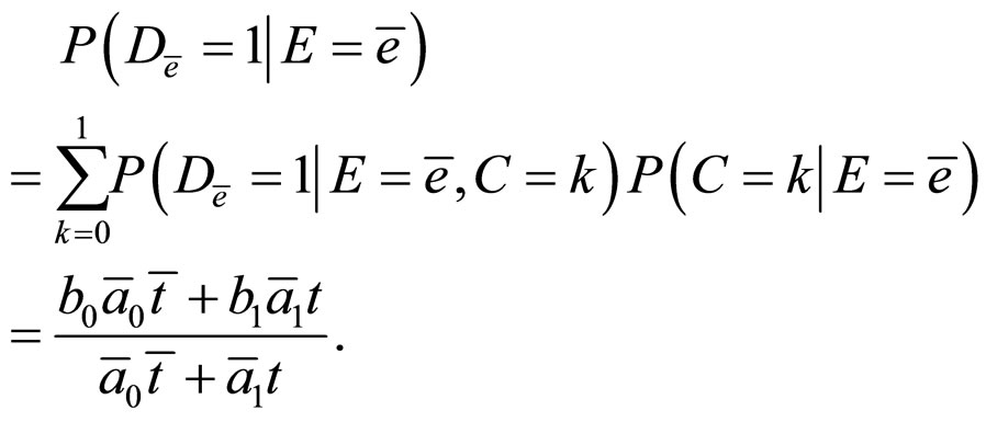
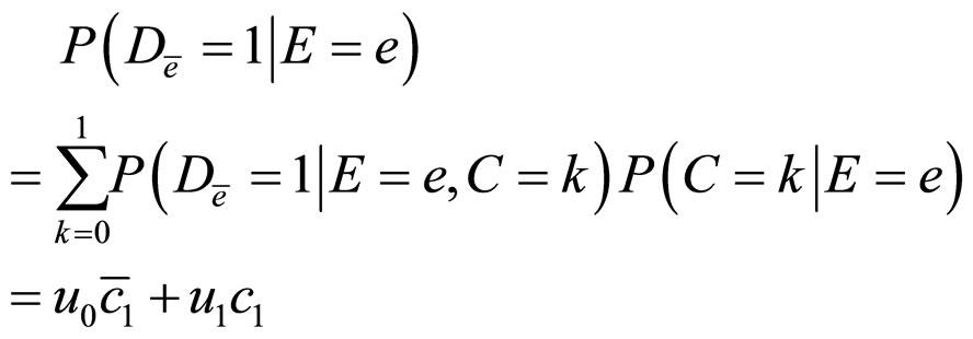
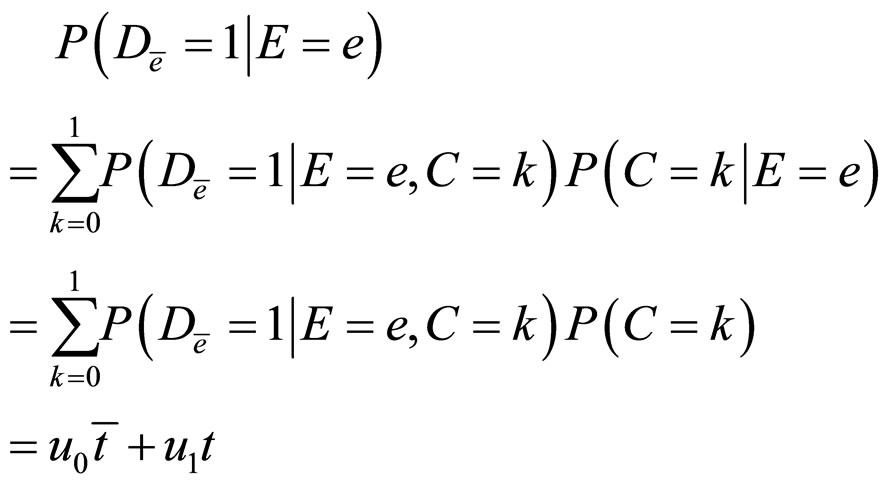
3.3. The Third Model
As shown in Figure 3, both  and
and  have effects on
 , and
, and .
.
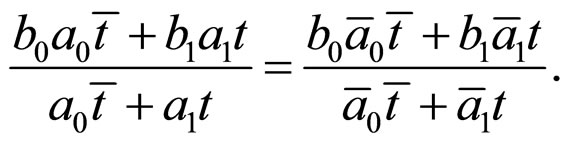
Denote,
where  can be observed from original data, but
  can not be observed because they are hypothetical proportions, or the probability with intervention [5].
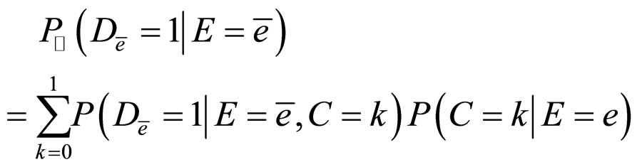
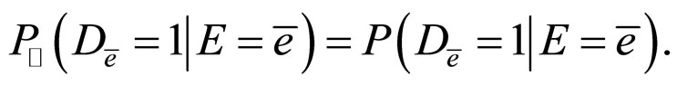
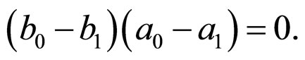
Then,


Then,
and,
 .
.
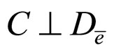
Hence, the covariate  is an irrelevant factor, but not a confounder, and it can not reduce confounding.
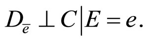
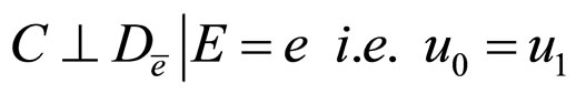
Using the above formulae, we translate each condition of (H) into parameter form, where  is naturally true in Figure 3.
1) 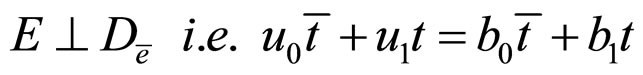
2) 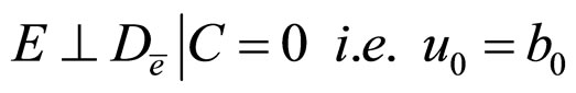
3) 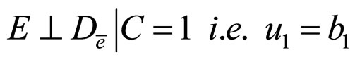
4) 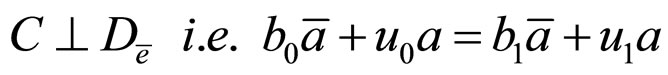
5) 
6) 
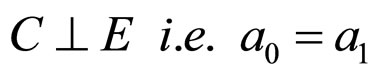
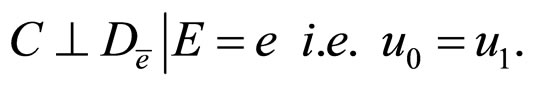
As discussed above, in the causal DAG Figure 3 with , the covariate
  is naturally an irrelevant factor. To keep the same expression as other DAGs, we have the following theorem.
Theorem 5. In the causal DAG of Figure 3 with , the covariate
  is an irrelevant factor.
Theorem 5 shows that in the causal DAG Figure 3, covariate  is always an irrelevant factor regardless of any adjustment or interventions on it.
Theorem 6. If one of the following conditions holds
a) 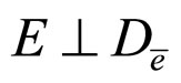
b) 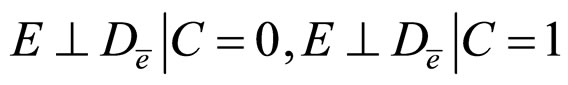
c) 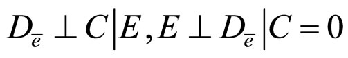
b) 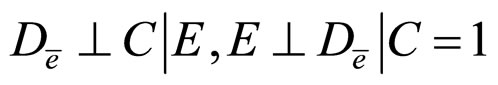
There is no confounding.
Proof.
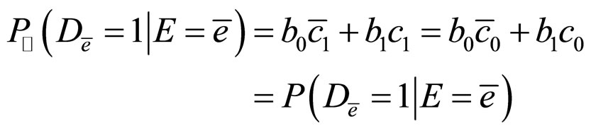
a) From the condition , we can obtain
Then,
b) From the conditions
 and
and we can obtain
 and
and .
.
Then,

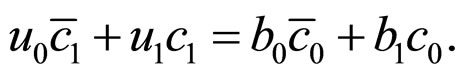
c) From the condition , we can obtain
 i.e.
i.e. ,
,
 i.e.
i.e. .
.
Furthermore,
 i.e.
i.e. 
Then,

d) The proof is similar to c). □
4. Conclusions
Using the formal definitions of confounder, non-confounding and irrelevant factor, we discuss the confounding of three kinds of three binary-variable counterfactual models in epidemiology studies and statistics, where the general causal DAG is involved in the discussion. The sufficient conditions of determining non-confounding and irrelevant factor in a three binary-variable causal DAG are discussed. Our work focuses on the general three binary-variable causal DAG, and no other variables are involved in discussion.
Furthermore, confounder and confounding are two different conceptions based on probability criteria, our discussions are definitely different from relative literatures, for example, [5,11,13]. In addition, the non-uniqueness of irrelevant factor and confounder in theory makes it more difficult to detect them and discuss the sufficient and necessary condition. The ancillary information (H) involved in our discussion is only a part of [5,13], hence we only obtain some sufficient conditions, another cause of this design lies in the thought that we want to discuss the causation along causal path. The sufficient and necessary condition discussion would be more complex as shown in our results. The future work will extend the three-variable counterfactual model to multi-variable counterfactual model. And, we will apply the theoretical results to the confounder detection in gene network.
5. Acknowledgements
This work is partially supported by National Natural Science Foundation of China for Youths (NSFC: 10801019). The author would like to thank the anonymous reviewer for the valuable comments and suggestions to make great improvement of this paper.