A Gauss-Newton Approach for Nonlinear Optimal Control Problem with Model-Reality Differences ()
1. Introduction
Many real processes are not linear in natural, so the actual model would not be necessary known. In addition to this, modeling the real process into a dynamical system could be an alternative solution plan. Since dynamical system has evolved over time, efficient computational approaches are highly demanded, and their development towards to optimize and control dynamical system is properly required. This situation imposes on obtaining the optimal solution of the real process enthusiastically. However, the difficulty level of solving the optimal control problems is increased with respect to the nonlinearity structure of dynamical systems. Simultaneously, the use of output measurement, especially from the industrial control applications [1] , becomes importance in constructing the corresponding dynamical system, which covers model predictive control [2] [3] [4] [5] , system identification [6] [7] [8] , and data-driven control [9] [10] [11] .
In fact, the solution methods of linear optimal control problem have been well-developed. Particularly, the linear quadratic regulator (LQR) technique is recognized as a standard procedure in solving the linear optimal control problems [12] [13] [14] [15] [16] . Recently, an efficient computational method, which is based on LQR optimal control model, is proposed to solve the nonlinear stochastic optimal control problems in discrete time [17] [18] [19] [20] . This approach is known as the integrated optimal control and parameter estimation (IOCPE) algorithm. It is an extension of the dynamic integrated system optimization and parameter estimation (DISOPE) algorithm [21] . The applications of the DISOPE algorithm have been well-defined in solving the deterministic nonlinear optimal control problem [22] [23] . By virtue of this, the IOCPE is developed, based on the principle of model-reality differences, for solving the discrete time deterministic and stochastic nonlinear optimal control problems.
Indeed, in both of these iterative algorithms, the adjusted parameters are introduced in the model-based optimal control problem. The aim is to calculate the differences between the real plant and the model used. These differences are then taken into account in updating the model used iteratively. Once the convergence is achieved, the iterative solution could approximate to the correct optimal solution of the original optimal control problem, in spite of model-reality differences. On the other hand, the use of the model output is an additional feature in the IOCPE algorithm [20] , which does not executed in the DISOPE algorithm.
Definitely, in this paper, the use of the output measurement, rather than adding the adjusted parameters into the model used, is further discussed. In our approach, the LQR optimal control model with the output measurement is simplified from the nonlinear optimal control problem. The differences between the output measurements, which are, respectively, from the model used and the real plant are defined. Follow from this, a least squares scheme is established. The aim is to approximate the output that is measured from the real plant in such a way that the output residual between the output measurements is minimized. In doing so, the linear dynamic system in the model used is reformulated and the control sequence is added into the output channel. Then, the model output is presented as input-output equations.
During the computational procedure, the control trajectory is updated iteratively by using the Gauss-Newton algorithm. As a result, the output residual between the original output and the model output is minimized. Here, the optimal control law is constructed from the model-based optimal control problem, which is not adding the adjusted parameters. By feed backing the updated control trajectory into the dynamic system, the iterative solution of the model used approximates to the correct optimal solution of the original optimal control problem, in spite of model-reality differences. Hence, the efficiency of the approach proposed is highly recommended. On the basis of this, it is highlighted that applying the least-square updating scheme for solving discrete-time nonlinear optimal control problems, both for deterministic and stochastic cases, are well-presented. See [24] for more details on stochastic case.
The rest of the paper is organized as follows. In Section 2, a discrete time nonlinear optimal control problem is described and the corresponding model-based optimal control problem is simplified. In Section 3, the construction of the feedback optimal control law is discussed. The output residual is defined in which a least-squares minimization problem for the model-based optimal control problem is formulated. The iterative algorithm based on the Gauss-Newton method is established, and the computational procedure is summarized. In Section 4, two illustrative examples, which are current converted and isothermal reaction rector problems, are demonstrated, and their results show the efficiency of the approach proposed. Finally, some concluding remarks are made.
2. Problem Statement
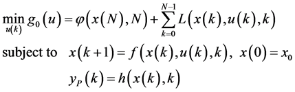
Consider a general discrete time nonlinear optimal control problem, given by
 (1)
(1)
where ,
,  and
and 
 are, respectively, control sequence, state sequence and output sequence,
  represents the real plant and
  is the output measurement, whereas
  is the terminal cost and
  is the cost under summation. Here,
  is the scalar cost function and
  is the initial state. It is assumed that all functions in Equation (1) are continuously differentiable with respect to their respective arguments.
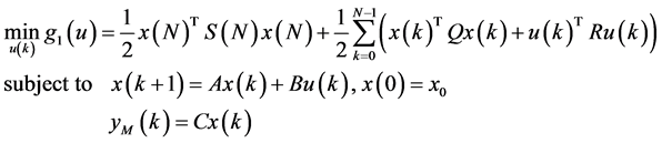
This problem, which is referred to as Problem (P), is complex. Solving Problem (P) would increase the computational burden and the exact solution might not exist due to the nonlinear structure of Problem (P). Nevertheless, in order to obtain the optimal solution of Problem (P), the linear model-based optimal control model, which is referred to as Problem (M), is proposed. This problem is given by
 (2)
(2)
where  is model output sequence,
  is a state transition matrix,
  is a control coefficient matrix, and
  is an output coefficient matrix, while
  and
and  are positive semi-definite matrices and
 ![]() is a positive definite matrix. Here,
is a positive definite matrix. Here, ![]() is the scalar cost function.
is the scalar cost function.
Notice that only solving Problem (M) would not give the optimal solution of Problem (P). However, by constructing an efficient matching scheme, it is possible to obtain the optimal solution of the original optimal control problem, in spite of model-reality differences.
3. System Optimization with Gauss-Newton Updating Scheme
Now, consider the following solution method on system optimization. Define the Hamiltonian function for Problem (M) as follows:
![]() . (3)
. (3)
Then, the augmented objective function becomes
![]() (4)
(4)
where ![]() is the appropriate multiplier to be determined later.
is the appropriate multiplier to be determined later.
3.1. Necessary Optimality Conditions
Applying the calculus of variation [12] [14] [15] [16] to the augmented cost function in Equation (4), the necessary optimality conditions are obtained, as shown below:
(a) Stationary condition:
![]() (5)
(5)
(b) Costate equation:
![]() (6)
(6)
(c) State equation:
![]() (7)
(7)
with the boundary conditions ![]() and
and![]() .
.
3.2. Feedback Optimal Control Law
According to the necessary conditions given in Equations (5) to (7), a feedback optimal control law could be constructed in which the optimal solution of Problem (M) is obtained. For this purpose, the corresponding result is stated in following theorem.
Theorem 1. For the given Problem (M), the optimal control law is the feedback control law defined by
![]() (8)
(8)
where
![]() (9)
(9)
![]() (10)
(10)
with the boundary condition ![]() given.
given.
Proof: From Equation (5), the stationary condition is rewritten as follows:
![]() . (11)
. (11)
Applying the sweep method [15] [16] , that is,
![]() , (12)
, (12)
and substitute Equation (12) for ![]() into Equation (11) to yield
into Equation (11) to yield
![]() . (13)
. (13)
Taking Equation (7) in Equation (13), and after some algebraic manipulations, the feedback control law (8) is obtained, where Equation (9) is satisfied.
From Equation (6), after substituting Equation (12) for ![]() into Equation (6), the costate equation is rewritten as follows:
into Equation (6), the costate equation is rewritten as follows:
![]() . (14)
. (14)
Considering the state Equation (7) in Equation (14), we have
![]() . (15)
. (15)
Apply the feedback control law (8) in Equation (15), and doing some algebraic manipulations, it is concluded that Equation (10) is satisfied after comparing the manipulation result to Equation (12). This completes the proof. ¨
Taking Equation (8) in Equation (7), the state equation becomes
![]() (16)
(16)
and the model output is measured from
![]() . (17)
. (17)
Hence, the solution procedure of solving Problem (M) is summarized below:
Algorithm 1: Feedback control algorithm
Data Given![]() .
.
Step 0 Calculate ![]() and
and ![]() from Equations (9) and (10), respectively.
from Equations (9) and (10), respectively.
Step 1 Solve Problem (M) that is defined by Equation (2) to obtain ![]() and
and![]() , respectively, from Equations (8), (16) and (17).
, respectively, from Equations (8), (16) and (17).
Step 2 Evaluate the cost function ![]() from Equation (2).
from Equation (2).
Remarks:
a) The data ![]() are obtained by the linearization of the real plant
are obtained by the linearization of the real plant ![]() and the output measurement
and the output measurement ![]() from Problem (P).
from Problem (P).
b) In Step 0, the offline calculation is done for ![]() and
and![]() .
.
3.3. Gauss-Newton Updating Scheme
Now, let us define the output residual by
![]() (18)
(18)
where the model output (17) is reformulated as
![]() . (19)
. (19)
Rewrite Equation (19) as the following input-output equations [25] :
![]() (20a)
(20a)
for convenience,
![]() (20b)
(20b)
where
![]() and
and![]() .
.
Notice that the matrix ![]() is the extended observability matrix, and the matrix
is the extended observability matrix, and the matrix ![]() is one type of block Hankel matrix [25] .
is one type of block Hankel matrix [25] .
Hence, consider the objective function, which represents the sum squares of error (SSE), given by
![]() . (21)
. (21)
Then, an optimization problem, which is referred to as Problem (O), is defined as follows:
Problem (O):
Find a set of the control sequence![]() , such that the objective function
, such that the objective function ![]() is minimized.
is minimized.
To solve Problem (O), consider the second-order Taylor expansion [26] [27] about the current ![]() at iteration
at iteration![]() :
:
![]() (22)
(22)
The first-order condition for Equation (22) with respect to ![]() is expressed by
is expressed by
![]() . (23)
. (23)
Rearrange Equation (23) to yield the normal equation,
![]() . (24)
. (24)
Notice that the gradient of ![]() is calculated from
is calculated from
![]() (25)
(25)
and the Hessian matrix of ![]() is computed from
is computed from
![]() (26)
(26)
where ![]() is the Jacobian matrix of
is the Jacobian matrix of![]() , and its entries are denoted by
, and its entries are denoted by
![]() (27)
(27)
From Equations (25) and (26), Equation (24) can be rewritten as
![]() . (28)
. (28)
By ignoring the second-order derivative term, that is, the first term at the left-hand side of Equation (28), we obtain the following recurrence relation:
![]() (29)
(29)
with the initial ![]() given. Hence, Equation (29) is known as the Gauss-New- ton recursive equation [26] [27] .
given. Hence, Equation (29) is known as the Gauss-New- ton recursive equation [26] [27] .
From the discussion above, the updating scheme based on Gauss-Newton recursive approach for the control sequence is summarized below:
Algorithm 2: Gauss-Newton updating scheme
Step 0 Given an initial ![]() and tolerance
and tolerance![]() . Set
. Set![]() .
.
Step 1 Evaluate the output error ![]() and the Jacobian matrix
and the Jacobian matrix ![]() from Equations (18) and (27), respectively.
from Equations (18) and (27), respectively.
Step 2 Solve the normal equation![]() .
.
Step 3 Update the control sequence by![]() . If
. If![]() , within a given tolerance
, within a given tolerance![]() , stop; else set
, stop; else set ![]() and repeat from Step 1 to Step 3.
and repeat from Step 1 to Step 3.
Remarks:
a) In Step 1, the calculation of the output error ![]() is done online, while the Jacobian matrix
is done online, while the Jacobian matrix ![]() might be done offline.
might be done offline.
b) In Step 2, the inverse of ![]() must be exist. The value of
must be exist. The value of ![]() represents the step-size for the control set-point.
represents the step-size for the control set-point.
c) In Step 3, the initial ![]() is taken from Equation (8). The condition
is taken from Equation (8). The condition ![]() is required to be satisfied for the converged optimal control sequence. The following 2-norm is computed and it is compared with a given tolerance to verify the convergence of
is required to be satisfied for the converged optimal control sequence. The following 2-norm is computed and it is compared with a given tolerance to verify the convergence of![]() :
:
![]() . (30)
. (30)
d) In order to provide a convergence mechanism for the state sequence, a simple relaxation method is employed:
![]() (31)
(31)
where![]() ,
, ![]() is the state sequence of the real plant and
is the state sequence of the real plant and ![]() is updated from (16).
is updated from (16).
4. Illustrative Examples
In this section, two examples are illustrated. The first example shows a direct current and alternating current (DC/AC) converter model [28] [29] , while the second example gives a model of an isothermal series/parallel Van de Vussue reaction in a continuous stirred-tank reactor [30] [31] . In these models, the real plants are in nonlinear structure and the single output is measured. Since these models are in continuous time, the simple discretization scheme with the respective sampling time is applied. The optimal solution would be obtained by using the approach proposed and the solution procedure is implemented in the MATLAB environment.
To be convenient, the quadratic criterion cost function, for both Problem (P) and Problem (M), is employed, that is,
![]()
where![]() ,
, ![]() and
and![]() .
.
4.1. Example 1
Consider the state space representation of a direct current/alternating current (DC/AC) converter model [28] [29] given by
![]()
![]()
![]()
with the initial![]() , where
, where ![]() and
and ![]() represent the current (in unit of ampere) and the voltage (in unit of volt) flow in the circuit, and
represent the current (in unit of ampere) and the voltage (in unit of volt) flow in the circuit, and ![]() is the control signal. This problem is referred to as Problem (P).
is the control signal. This problem is referred to as Problem (P).
The discrete time model of Problem (M) is formulated by
![]()
![]()
for![]() , with the sampling time
, with the sampling time ![]() minute.
minute.
The simulation result is shown in Table 1. The initial cost of 0.0429 unit, which is the cost function value for Problem (M), is calculated before the iteration. After five iterations, the convergence is achieved. The final cost of 110.8926 units is preferred instead of the original cost of 1.0885 × 10³ units. This reduction saves 89.8 percent of the expense. The value of SSE of 7.647011 × 10?12 shows that the model output is very close to the real output. Hence, the approach proposed is efficient to obtain the optimal solution of Problem (P).
Figure 1 shows the final control trajectory, which is used to update the model output, in turn, to approximate the real output trajectory. From Figure 2, it can
![]()
Figure 2. Final output (?) and real output (+) trajectories.
![]()
Table 1. Simulation result for Example 1.
be seen that both of the output trajectories are fitted each other with the smallest value of SSE.
Figure 3 shows the control trajectory, which is applied in the real plant. With the matching scheme that is established in the approach proposed, the final state trajectory tracks the real state trajectory closely, as shown in Figure 4.
Figure 5 and Figure 6 show the initial trajectories of control and state, respectively. They are the optimal solution of Problem (M) before the Gauss- Newton updating is applied.
The differences between the real output and the model output, which are after and before iteration, and are shown in Figure 7 and Figure 8, respectively. These
![]()
Figure 4. Real state (+) and final state (?) trajectories.
model-reality differences reveal the applicability and reliability of the approach proposed, where the output error is minimized definitely.
4.2. Example 2
Consider the dynamical system of an isothermal series/parallel Van de Vussue reaction in a continuous stirred-tank reactor [30] [31] :
![]()
![]()
![]() with the initial
with the initial![]() , where
, where ![]() and
and ![]() are, respectively, the dimensionless reactant and product concentration in the reactor, and
are, respectively, the dimensionless reactant and product concentration in the reactor, and ![]() is the dimensionless dilution rate. Let this problem as Problem (P).In Problem (M), the model used is presented by
is the dimensionless dilution rate. Let this problem as Problem (P).In Problem (M), the model used is presented by![]()
![]() for
for![]() , with the sampling time
, with the sampling time ![]() second.Table 2 shows the simulation result, where the number of iteration is 5. The
second.Table 2 shows the simulation result, where the number of iteration is 5. The
![]()
Figure 8. Output error before iteration.
![]()
Table 2. Simulation result for Example 2.
implementation of the approach proposed begins with the initial cost of 12.6916 units. During the iterative procedure, the convergence is achieved with giving the final cost of 543.1649 units. This shows a reduction of 99.8 percent of the saving cost from the original cost of 3.0122 × 10⁵ units. The value of SSE of 1.587211 × 10?12 indicates that the approach proposed is efficient to generate the optimal solution of Problem (P).
The graphical result in Figure 9 and Figure 10 shows, respectively, the trajectories of final control, final output and real output. The final control is stable and this stabilization manner makes the steady state of the final output occurred at 1.2324. Moreover, the final output fits the real output very well.
Figure 11 and Figure 12 show the trajectories of control and state in the real plant. With this control trajectory, the state trajectories are converged to 2.8250 and 1.2324, respectively. In addition, by using the approach proposed, this steady state is tracked closely by the final state trajectory.
The initial trajectories of control and state are shown, respectively, in Figure 13 and Figure 14. They are the optimal solution of Problem (M) before the Gauss-Newton updating scheme is employed.
Figure 15 and Figure 16 show the differences between the real output and the model output, respectively. These differences are the output error, which is minimized apparently.
![]()
Figure 10. Final output (?) and real output (+) trajectories.
![]()
Figure 12. Real state (+) and final state (?) trajectories.
4.3. Discussion
From Examples 1 and 2, the structures of Problem (M) and Problem (P) are clearly different. Solving Problem (M) with taking the Gauss-Newton updating scheme into consideration provides us the iterative solution, which approximates to the correct optimal solution of Problem (P), in spite of the model-re- ality differences. The results obtained are evidently demonstrated in Figure 1 and Figure 16. Hence, the applicability of the approach proposed is significantly proven.
5. Concluding Remarks
In this paper, an efficient computational approach was proposed, where the least squares scheme is established. In our approach, the model-based optimal control problem is solved in advanced. Consequently, the feedback control law, which is constructed from the model used, is added in the output measurement. Through optimizing the sum squares of error, the Gauss-Newton updating scheme is derived. On this basis, the control trajectory is updated repeatedly during the computational procedure. By feed backing the updated control trajectory into the dynamic system, the iterative solution of the model used approximates to the correct optimal solution of the original optimal control problem, in spite of model-reality differences. For illustration, two examples were studied. Their simulation results and graphical solutions indicated the applicability and reliability of the approach proposed. In conclusion, the efficiency of the approach proposed is proven.
Acknowledgements
The authors would like to thanks the Universiti Tun Hussein Onn Malaysia (UTHM) and the Ministry of Higher Education (MOHE) for financial supporting to this study under Incentive Grant Scheme for Publication (IGSP) VOT. U417 and Fundamental Research Grant Scheme (FRGS) VOT. 1561. The second author was supported by the NSF (11501053) of China and the fund (15C0026) of the Education Department of Hunan Province.