Analysis of the Effect of Subgroup Size on the X-Bar Control Chart Using Forensic Science Laboratory Sample Influx Data ()
1. Introduction
The forensic science laboratory (FSL) studied comprises of three disciplines (forensic biology and DNA, forensic chemistry and forensic toxicology), which receive, examine, analyze and reports on evidence submitted in criminal cases from all over Tanzania. The FSL is the sole legally authorized laboratory to examine evidence submitted by any Governmental agency investigating a criminal offense. Crime scenes are the primary point of detection, collection, and preservation of evidence, before submission to the FSL. All of the methods and processes employed at a crime scene are geared toward stopping the clock, i.e., keeping the scene and the evidence as much as it was when the crime was committed as possible until it can be recorded and documented. The evidence received is viewed in the context of the crime, the persons involved, and the environment (both physical and temporal). Science applied at the scene can generate data for later analysis, provide quicker answers, and facilitate better analysis in the laboratory. Currently, the sample influx is overwhelming, which require statistical analysis and decision making.
The FSL studied is part of a dynamic multi-disciplinary organization devoted to the ideals of excellence that provides leadership to advance forensic science and its application to the police investigation unit and legal system and other services offered by the organization. Currently, the FSL has undertaken studies to debottleneck the challenges including extended turnaround time (TAT), large number of case files submitted, large number of evidence or samples submitted per case file, defined in this study as sample influx data, financial and administrative hurdles, and human resource challenges. The SIF data shows strong variations with time, from case file to another and among the three disciplines, posing a challenge to the FSL performance.
This paper focuses on the statistical time series analysis techniques on SIF data and introduces application of x-bar control chart technique as a tool for identifying uncommon occurrences of high sample influx so that causes can be identified and action can be taken to keep the sample management process under control.
Higher SIF to FSL affects the sample management process. Demand on human resource, funds for reagents and other consumables, high equipment utilization rate and repair, administrative burdens (documentation, quality control) are among the effects of high SIF to the FSL management. Moreover, high demand on utilities (water, electricity, compressed gases, cooling and storage facilities, etc.) and increased laboratory space requirements necessitate a closer look at SIF data so that decisions can be made based on scientific evidence. Other effects of high SIF include high report volumes and writing and review time, payment of extra hours and demand for expert witness sessions’ preparation time for analysts.
Antagonistic scenarios prevail between crime scene exhibit collection and FSL sample analysis and reporting. While crime scene investigation demand collection of as large number of evidence as possible (which leads to elevated SIF), the FSL enters a state of management surge in trying to accommodate high SIF leading to extended TAT, which forms a large component of reasons for complaints by its clients (investigation, prosecution and judiciary).
The SIF data can be analyzed using time series analysis techniques. Statistical analysis techniques tend to unfold hidden details of the inherent process that are usually contained in the time series. Those details are necessary in order to build critical understanding of the system or process being assessed. With increased understanding of the process, control action and decision making become easy for elimination of the causes of process instability.
There exists several time series analysis techniques employed in analyzing engineering systems. This study used x-bar control charts to signal problems in either crime scene management techniques, investigator skills, change of national or regional crime profile, the need for re-planning for human resources, space, equipment and technology acquisition, budget review process, or funding re-allocation. The x-bar and range charts are the most common control charts used in measuring continuous data well known as fundamental tools for displaying the range of variability inherent to a process [1] [2] [3] [4] . This is also referred to as statistical process control (SPC).
Application of several rules to the same set of data is referred to as multi-rule analysis. The rules can be implemented separately (as in this work) or in combination [5] . The advantage of multi-rule quality control procedures include minimization of false out-of-control detection, while at the same time maintaining high out of control detection. In this study, the multi-rule application was done by selecting individual rules with different levels of violation detection, then applying them separately, while other researchers apply them jointly to maximize detection levels, so called stringent process control. Thus, multi-rules optimize both sensitivity and specificity of the quality control process, and were implemented to build an insight understanding of the behavior of the evidence or sample reception system and the power of the control charts [6] [7] [8] . This study utilized a computer code to identify violations using several rules applied separately different from simultaneous application of multi-rules [9] [10] .
Research on SPC is wide in industry and medical laboratories, but has not been focused in forensic science laboratories for cost and quality improvements. While FSL’’s reports contribute strongly in the judiciary system, the use of control chart as quality control tool is an important research area. The purpose of this research was to provide a scientific basis for choosing rational subgroup size, given an acceptable range of 2 to 25. None of the researchers dealt in depth on the scientific identification of rational subgroup size.
2. Literature Review
The primary use of x-bar control charts is to help in determining whether or not the process in question is stable [3] [4] [11] . In general, “stable” refers to a state of statistical control, a condition which exists when the process is affected by only common or random variation, that is, variations inherent in the process and not caused by unusual influences. In this study, control charts were used to signal unusual occurrence of SIF, and hence allow for re-examination of case files in the respective subgroups which exceeded the upper control limit. A special cause is present in the process if any points fall above the upper control limit or below the lower control limit, the so called Rule #1, giving the number of exceedances as out-of-control points. Action should be taken to find the special cause and permanently remove it from the process by making changes in the investigation techniques a problem which is outside the scope of FSL.
Other rules use the zones to test for process stability, called zone tests (Rule #2 to #4). The zone tests are valuable tests for enhancing the ability of control charts to detect small shifts quickly. In this study, Rule #2 to #4 were implemented based on zone tests while Rule #5 which is based on trending behavior was also implemented in order to build understanding on the ability of the control charts. The first step in using these tests is to divide the control chart into zones, by dividing the area between the average and the upper control limit into three equally spaced areas. The locations of the lines depend on standard deviation and a factor of the latter to be added to the grand mean. This is then repeated for the area between the average and the lower control limit.
The x-bar control charts consist of three zones, that is, A, B, and C. There is zone A for the top half of the chart and a zone A for the bottom half of the chart. The same is true for zones B and C. The charts are normally based on 3 sigma limits of the variable being plotted. This method works perfectly for a normally distributed process [11] . Thus, each zone is normally one standard deviation in width. For example, considering the top half of the chart, zone C is the region from the average to the average plus one standard deviation. Zone B is the region between the average plus one standard deviation and the average plus two standard deviations. Zone A is the region between the average plus two standard deviations and the average plus three standard deviations. In this work, a test was conducted to assess the effect of number of sigma on the control charts characteristics, and a choice of the control limits made based on suitability of the control chart in detecting the process instability, because the studied process does not follow a normal distribution, as shown later. The control limits (defined for the statistic that is being plotted) are statistically determined by observing process behavior, providing an indication of the bounds of expected process behavior [1] [12] . The fluctuations of the points between the upper and lower control limits are due to the variation that is intrinsic (built in) to the process (that is, sample submission to the forensic science laboratory). These variations are due to common causes. Although we do not know exactly what these causes are, they are specific to each crime scene and their effect on the process seems to be consistent over time. Thus, if the process is in control, the vertical location of subgroup average value that lies between the control limits is not useful information. When points exceed the control limits, we assert that the process must have shifted, since the chance of this happening is so small. Due to averaging within each subgroup, any point outside the control limits is attributed to special causes. It should be noted that a point falling beyond the upper control limit is the average of all values in that subgroup, such that there must be an unusual situation in the respective subgroup time interval worth examining in details using the subgroup data and taking remedial action in the real process. A key value of the control chart is to identify the occurrence of such special causes so that they can be identified and removed, leading to a reduction in overall process variation.
The limits are determined by estimating the short-term variation in the process, which are then used in defining process stability (or process control). The short-term variation provides a good model (or estimate, or prediction) of the longer-term variations because if short term variation remains under control, eventually the long term variations will be under control or stable. The short-termism arises from the choice of the subgroup size. This is the most critical component towards effective use of these control charts, yet one of the most overlooked. This paper examines the effect of subgroup size on the performance of the control chart as a statistical tool.
This paper presents a new criterion on choosing subgroup size for the data in hand. As stated above, each subgroup represents a snapshot of the process at a given point in time. The x-axes of the x-bar control chart are time-based, so that the charts show a history of the exhibit or sample receiving process. X-bar charts are efficient at detecting relatively large shifts in the process average, typically shifts of ±1.5 sigma or larger. The larger the subgroup, the less-sensitive the chart will be to shifts in the process.
Different researchers use subgroup sizes depending on convenience of data collection, and limitations posed by literature values of subgroup size. The key to successful control charts is based on formation of rational subgroups. Control charts rely upon properly selected subgroups to estimate the short-term variations in the process. The short-term variations are then used to predict the longer-term variation defined by the control limits, which differentiate between common and special causes of variations. A rational subgroup is simply a sample in which all of the items are produced under conditions in which only random effects are responsible for the observed variation. This study critically investigates the ability to identify process instability at a wide range of subgroup sizes for the same data set, that is, SIF data.
This paper deals with an approach for choosing the proper subgroup size for control charts. Other researchers used ANOVA for testing that the process mean is in control and Bartlett’s test for testing that the process variance is in control [13] . The subgroup sizes were created assuming that several conditions for subgroup properties were satisfied. It was assumed that the observations within a subgroup are from a single, stable process, with few special causes within subgroups, to have small variations within subgroups relative to the variation between subgroup averages. Presence of large variations within subgroup forces the control limits to be too far apart, resulting in a lack of sensitivity to process shifts. However, the control limits depend on characteristics of the overall data set based on standard deviation or average range [11] [14] .
The purpose of x-bar control charts is to detect significant process changes when they occur. In general, charts that display averages of data like x-bar charts are more useful than charts of individual data points. Charts of individuals are not nearly as sensitive as charts of averages at detecting process changes quickly. X-bar charts are far superior at detecting process shifts in a timely manner, and the subgroup size is a crucial element in ensuring that appropriate chart signals are produced [15] .
Often, the subgroup size is selected without much thought. A subgroup size of 5 seems to be a common choice. If the subgroup size is not large enough, then meaningful process shifts may go undetected. Based on the limitations over batch completion time, a value of k = 11 was used for saccharification temperature, pH and Brix data control charts [11] . On the other hand, if the subgroup size is too large, then chart signals may be produced from insignificant process shifts. The key is to specify a subgroup size so that significant shifts (from a practical perspective) are detected with high probability and that insignificant shifts are unlikely to produce a signal [16] [17] . The observations within the subgroups are independent, implying that no observation influences, or results from, another. If observations are dependent on one another, the process has autocorrelation which causes the within subgroup variation to be unnaturally small and a poor predictor of the between subgroup variation. The small within subgroup variation forces the control limits to be too narrow, resulting in frequent out of control conditions or false violations.
3. Methodology
3.1. Data Collection and Organization
The SIF data comprised of details per case files received in each calendar year from January to December. Each request submission contains a different number of samples or evidence, referred to as case file. Since the sample influx data was collected from recorded sample receiving datasheets, as the samples were being received, then the subgroups are formed from observations taken in a time-ordered sequence, i.e., from a time series of sample influx, or SIF, denoted as S(t). In other words, subgroups were formed using a snapshot of the process over a small window of time, and the order of the subgroups would show how those snapshots vary in time. Given that 629 case files were received in 260 working days (SIF2014 with highest case files), at an average of 3 case files per day, a value of k = 2 or 3 spans a time window of one day. Thus, values of k higher than 3 are recommended for SIF data. On the other extreme, a maximum value of k = 25, on the other extreme, is equivalent to 8.33 working days, which is within 2 weeks. Thus, most of the values of k used in this study investigate variations in a time window of 1 to 2 weeks, which can be too long maximizing the chance of special causes. Thus, for sample influx data, one week or 5 days should be sufficient, that is k = 5 × 3 = 15 maximum. In this case, analysis of k = 2 to 15 to provide a time window of 5 working days in a week is recommended. The details of the SIF data used in this study including number of case files received at FSL and the corresponding statistics is summarized in Table 1.
3.2. Choice of Subgroup Size
This study was mainly focused on characterizing stability of the system as the subgroup size was increased from 2 to 25. Given a time series of sample influx data, S(t), of length Npt, as the number of subgroups, k, is changed the number of groups for which average values are determined and compared with control limits changes as per Equation (1):
 (1)
(1)
Since only complete columns of subgroups can be processed, the incomplete subgroups were truncated leading to slight variations in the grand mean,  and standard deviation. However, the analysis was still valid since each value of k gives a complete and independent x-bar control chart, assessed for violation using five Rules. The choice of number of subgroups Nsg or the size of subgroups, k (where Npt = Nsg × k) affects the resulting control chart in terms of number of points that exhibit out of control behavior, the percentage of the out of control points, and also the control limits UCLx, LCLx, as well as the zone demarcations, XA and XB, as shown in Table 2, for Npt = 620.
![]()
Table 1. Statistical analysis of the SIF data (samples per case file) used in this study.
![]()
Table 2. Effect of increasing subgroup size on control chart parameters and process stability (SIF2014).
3.3. Control Chart Characterization Parameters
The main purpose of x-bar control chart is to identify and count the number of out-of-control points (OCP) denoted as Nocp, observed above the upper control limit, UCLx, using Equation (2):
 (2)
(2)
where n is the number of multiples of sample sigma above the grand mean to determine the upper control limit. For a normal distribution, n = 3. However, for a distribution away from normal, it is wise to establish the coefficient n before a control chart can be used to assess stability of the process. In the literature, the value of n used to set the control limits is usually stated in the rules to be used, such as 2of32s as introduced in Westgard Rules.
3.4. Parameters Determined
The count of number of times any rule was violated, denoted as OCP, was established based on the selected value of n = 1.0 for setting the control limits, as per Equation (3):
 (3)
(3)
This led to the three zones separated by the lines XA and XB, as per Equations (4) and (5):
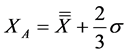 (4)
(4)
and
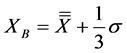 (5)
(5)
The percent of out-of-control points for different control-chart interpretation rules for a given number of subgroups, Nsg, (that is, for each value of k) was determined using Equation (6):
 (6)
(6)
3.5. Application of Multi-Rules to the X-Bar Control Chart
Literature shows that there are times when control limits are set using 3σ, 2σ or 1σ [11] [14] including use of control chart constant multiples of R-bar [11] . The question is, when to use control limit other than 3σ. During preliminary work, test for effect of n or Nocp and Pocp were conducted for n ranging between 0 and 3, while varying k, and a choice of n = 1.5 was made.
Detailed analysis of control charts uses a collection of rules to asses for condition leading to denoting the process (from which a time series originates) as out of control or unstable [11] . The rules which were used in the analysis are summarized in Table 3.
Rule #1 signifies process control rule where a violation was counted as Nocp when a subgroup average exceeds the upper control limit set as per Equation (3), where n = 1, which is different from a usual action or rejection limit on Shewhart control chart that uses Equation (2) with n = 3. The decision to use n = 1 was reached through sensitivity analysis for SIF data, as shown in Figure 1. Based on results shown in Figure 1, the numbers of points beyond  and
and  are already very small (equal to 1) for k ≥ 10, indicating that, further analysis of the effect of k will be restricted. By virtual of the maximum value being above UCLx, it is evident that Nocp will be higher than 1, allowing analysis of Nocp with k except at k = 25. Thus, this study used n = 1.
Rule #2 was implemented using a count of times at least 2 points out of 3 exceed XA. This count was established by summation of cases where all three points (Rall3), first and second points (R1&2), first and third points (R1&3), or second and third points (R2&3) were observed to exceed XA. Whenever Rule #2 is
![]()
Table 3. Rules for assessing stability using control charts.
![]()
![]()
Figure 1. Sensitivity analysis of the effect of n and k on control limits, UCLx and number of violations, Nocp.
violated, the count of number of violations is increased by unity, such that the total number of violations can be expressed as per Equation (7):
 (7)
(7)
where the exponent denotes rule number.
Rule #3 was implemented by counting number of times the following scenarios were detected among the average values for each subgroup: the 1st to 3rd points (R1to3), 2nd to 4th points (R2to4), or 3rd to 5th points (R3to5) are above XB. Thus the rule is violated whenever any of these scenarios is observed, such that, the total number of possible violations is the sum of three possibilities, defined using Equation (8):
 (8)
(8)
Rule #4 was implemented by assessing when eight consecutive average values of the subgroups were above XB [14] , a sequence of which is denoted as Q(p) for 
Let ,
, ![]() ,
, ![]() ,
, ![]() ,
, ![]() , be consecutive values of Q(p) starting at point p in the series. If
, be consecutive values of Q(p) starting at point p in the series. If
![]() (9)
(9)
where symbol “Λ” represents an “AND” operator, then Rule #4 is violated and Nocp is increased by 1, until all cases where the condition is fulfilled are counted. This is denoted as 8x in multi-rule implementation. When condition stipulated in Equation (9) is fulfilled, the number of OCP or violations are counted, denoted as Rall8, expressed as per Equation (10):
![]() (10)
(10)
Rule #5 was implemented by assuming that a sequence of Q(p) values, such that![]() ,
, ![]() ,
, ![]() ,
, ![]() ,
, ![]() , satisfies the condition given in Equation (11):
, satisfies the condition given in Equation (11):
![]() (11)
(11)
This implies that six consecutive points in Q(p) series steadily decreases [14] . This is denoted as 6 T in the multi-rule implementation. Thus, the count of violations is increased by unity until all cases where the conditions are fulfilled are counted, as per Equation (12):
![]() (12)
(12)
Since all the rules were applied separately to the sample influx data, Figure 2 shows the flow chart for implementation of the rules.
3.6. Application of a Computer Code
Based on results shown in Figure 1 and the multi-rule implementation in Figure 2, it is evident that there are many variations of violations in the characteristics of the control chart, which require a computers code to capture the violations and keep counts as k is varied [3] [6] [7] [8] [9] . A FORTRAN computer code
![]()
Figure 2. Flow chart of multi-rule implementation adopted in this study.
was implemented to read the original time series, S(t), create subgroups automatically, and create the upper and lower control limits, followed by calculating the averages for each subgroup and performing violations detection.
While the x-bar control chart rules might be used differently in different applications, it is important to note that these rules are intended to provide evidence of out-of-control process and not conclusive proof. Once out-of-control points are observed in the data, causes are investigated in the real or physical system, remedies made and observation on the effect of remedial action investigated once again.
With such wide range of variations in control chart characteristics, a FORTRAN code was created to read the time series data and perform the analysis of detecting instability using the above rules and mainly testing the effect of subgroup size, k, stating from 2 to 25. The parameters assessed for OCP were related to k using power and exponential functions of different coefficients and indices.
4. Results and Discussion
4.1. Sample Influx Time Series
The sample influx data recorded chronologically for 629 case files received into the FSL in the year 2009, 2014 and 2015 is presented in Figure 3. The sample influx fluctuated from 1 to above 600 samples per case file, with spikes of very high influx occurring randomly with time. This tendency of random sharp rise affects strongly the operations and performance of FSL as it impacts human resource and staffing requirements, supplies, extended TAT and longer working hours for employees. To answer the question, whether the influx fluctuations are still statically under control, control charts were suggested and implemented. The higher values of S(t) on the other hand, affects the performance of FSL strongly, due to extended TAT in handling large number of samples, high consumption of reagents and other consumables.
4.2. Probability Distribution Function of the SIF Data
When the data was tested for underlying nature of distribution, it was evident that the SIF data is not normally distributed. The probability distribution functions (PDFs) show high positively skewed distributions with skewness = 5.69, 7.48 and 7.06 and very high kurtosis values = 41.18, 73.42, and 63.17, for SIF2009, SIF2014 and SIF2015, respectively, as shown in Figure 4. The longer tails on the right for all the three PDFs signify that, each year very high values of SIF exist at lower frequencies as indicated by few longer peaks in Figure 3. Very higher SIF values than 100 samples per case file were observed, indicating case files with higher public interest. The PDF of SIF2009 data shows a slight difference from the recent data sets, of having a bimodal behavior, attributable to effective training offered by the FSL to the investigation team. Also, in 2009, the FSL was in infant stages of implementing Human DNA Regulation Act and the corresponding test procedures including paternity testing (for which three samples
![]()
![]()
![]()
Figure 3. Time series of sample influx data.
![]()
Figure 4. Probability density functions (PDFs) of the SIF data from three years.
are required) which manifests in the peak at S(t) = 3 samples for SIF2014 and SIF2015. The peaks at S(t) = 1 signifies case files where a single sample was submitted to the FSL, which occur at highest frequency, especially for SIF2009. Despite the difference in number of case files received (SIF2014 and SIF2015 data sets) results show similar behavior compared to SIF2009, all of which are not normal distributions.
4.3. X-Bar Charts Characterization Based on 3σ Control Limits
4.3.1. Sample X-Bar Control Charts at Different Subgroup Sizes
The effect of sub-group size was initially investigated by plotting control charts at selected interval of subgroup sizes. In each case, different control limits and zonal demarcations of the x-bar charts were identified. Figure 5 shows the sample control charts for k = 5, 10 and 15, respectively. In σ, horizontal axis is the subgroup number, Sbg, while vertical axis is the subgroup average values, Q(p). The number of bunches or subgroups of case files decreased from 124, 62, and 41 when k was increased from 5, 10 and 15, respectively. It is notable that the number of out-of-control points based on ![]() decreased from 12 at k = 5 to 8 at k = 10, and decreased further to 3 at k = 15. This shows clearly that the subgroup size is an important parameter of the x-bar control chart for proper decision making in identifying process instability.
decreased from 12 at k = 5 to 8 at k = 10, and decreased further to 3 at k = 15. This shows clearly that the subgroup size is an important parameter of the x-bar control chart for proper decision making in identifying process instability.
Figure 5 uses the same vertical scale in order to compare the number of Nocp, but Also to show that the Q(p) values decreases with k. For instance, at k = 5, the maximum value of Q(p) was 182 samples per case file, while at k = 10 the maximum value was 120 and down to 50 at k = 15. It should also be noted that the shape of the Q(p) curves at different values of k remains the same (Figure 5), but varying in vertical span only. Results show that changing k, the number of subgroups changed as well as the upper and lower control limits of the charts, showing that the setting of the control chart need to be well scrutinized in order to portray the meaningful results.
4.3.2. Analysis of the Effect of Subgroup Size on X-Bar Chart Characteristics
The resulting changes in the control chart parameters are listed in Table 2 for different values of k. Based on results reported, control charts must be used and interpreted with care. The effect of subgroup size on the useful control charts parameters is well stipulated in Table 2 for n = 1, 2, 3 although detailed analysis used n = 1 only. It is also noted that Pocp does not decrease with k, like Nocp because the denominator Nsg is also decreasing. The results of out-of-control points shown in Table 2 are based on simple basic concept of control charts, that is, when the average values of Q(p) exceeds the UCLx.
Other characteristics of the control chart that depend on the subgroup size include ![]() (where if the time series data is truncated to fit the complete subgroups, especially at higher values of k), UCLx, LCLx, and span between limits, SPx, as shown in Figure 6. With all values of LCLx being negative, this analysis did not use such limits. Results show that the control limits shrink when k increases, so
(where if the time series data is truncated to fit the complete subgroups, especially at higher values of k), UCLx, LCLx, and span between limits, SPx, as shown in Figure 6. With all values of LCLx being negative, this analysis did not use such limits. Results show that the control limits shrink when k increases, so
![]()
![]()
![]()
Figure 5. X-bar control charts of SIF data at three different subgroup sizes (data from SIF2014) using 3σ limits above the grand mean.
that SPx drops from 46.87 at k = 5 to 40.39 at k = 15. Further increase in k will result into even narrower area between units since the standard deviation decreases continuously.
Based on the nature of S(t) and Q(p), that is the number of samples per case file, negative control limits were excluded in the analysis, and only x-bar, UCLx, XA, and XB were used in detecting violations.
![]()
Figure 6. Effect of subgroup size on x-bar chart characteristics (for SIF2014 with n =3).
4.3.3. Comparison of X-Bar Charts for Different SIF Data
While Figure 5 shows the control charts at different subgroup sizes, k, the need to compare the behavior for SIF data from different years revealed the behavior of the SIF data on a control chart, as shown in Figure 7, for k = 5. Based on Figure 7 and Rule #1 which can be implemented manually by counting exceedances over UCLx as violations, Table 4 shows the detailed analysis of the control charts based on Rule #1.
Figure 7 and Table 4 show clearly that there is a wide variation in control chart limits between SIF data series, depending on the statistics embedded in the data sets from different years, being highest for SIF2014. Moreover, the span between control limits, SPx, was narrowest for SIF2009 compared to the rest of the data sets. The number of violations observed were different, being 13, 12 and 8 leading to Pocp = 17.57%, 9.68% and 8.0% for SIF2009, SIF2014 and SIF2015, respectively. It is evident that the number of violations (Nocp) and percent of violations (Pocp) decreased with time. The changes observed in the Pocp can be attributed to the effectiveness of the training for the investigation team on sample collection, storage and transportation prior to submission to the FSL.
4.4. Probability Density Functions for the Subgroup Average Values
Several series of the subgroup average values, Q(p), equal in number to Nsg, were determined and recorded for further statistical analysis. The probability density functions (PDFs) at selected values of subgroup sizes, k = 2, 5, 10, 15, 20 and 25, are plotted in Figure 8. It was observed that the data is characterized by positive skewness with longer tails towards the right. The values of skewness decreased from 5.12 to 1.44 when k was increased from 2 to 25. The plots reveal a slight decrease in the scatter of Q(p) values, or an increase in uniformity of the average values, as the value of k increases, such that the standard deviation decreased from 35.3 to 15.0 while the range of the Q(p) values dropped from 328.5 to 51.6.
![]()
![]()
![]()
Figure 7. X-bar control charts of SIF data (at k = 5 and n = 3).
![]()
Table 4. Summary of the detailed analysis of control charts for SIF data at k = 5.
Despite the similarity in the shape of the PDFs, they differ in terms of frequency or vertical axis for which the minimum observed frequency increases with k from 1% when k = 2% to 4% when k = 25, showing that the Q(p) approaches a normal distribution when k increases. There is also a shift along horizontal axis when k increases with the tail at lower values of Q(p) diminishing when k increases. Such observation has been reported in literature especially for data exhibiting normal distribution.
It is evident that increasing k leads to a more uniformity among the Q(p) values due to averaging effect as subgroup size increases. Moreover, the span and the maximum value of Q(p) decreases with k. The changes in statistics between the original time series data and the Q(p) can be seen by comparing the statistical values as shown in Table 5.
It was observed that as the subgroup size increases the standard deviation of
![]()
Table 5. Statistical analysis of the Q(p) data from SIF2014.
the distribution of averages decreases. Specifically, the relationship shown in Table 5 relates the standard deviation of averages to the standard deviation of individuals or S(t) as the subgroup size increases.
Figure 9 shows a plot of cumulative probability distribution functions of the Q(p) series data for k = 2, 5, 10 and 15 and that of the original SIF data, denoted as S(t) for SIF2009 and SIF2015. The plots show the properties of the Q(p) data using the differences in loci. While the span of the Q(p) values decreases at higher values of k, a great similarity is observed in the shape of the cumulative functions, showing that the SIF data emanates from a distinguished and unique system determined by control factors constantly governing the sample collection at crime scene and its management before submission to the FSL.
4.5. Variation of Number of Violations with Subgroup Size
Figure 10 shows the variation of the number of violations or number of OCP with subgroup size for different rules implemented in this analysis. All rules reveal a clear decreasing tendency for violations when k increases. This is attributed to the decrease in span between the control limits when k increases.
![]()
![]()
Figure 9. Cumulative probability functions of subgroup averages, Q(p), for different subgroup sizes using SIF data.
![]()
Figure 10. Variation of number of violations with subgroup size, k, for the five control chart rules using SIF2014 data set (using n = 1).
However, Rules #2 and #3, shows poor relationship between number of violations with subgroup size as the fluctuations were observed to increase with k. Thus, further analysis was conducted for Rule #1, #4 and #5.
It should be noted that Rules #2, #3, #4 and #5 can lead to Nocp higher than Nsg due to the fact that one point can be counted several times as long as the neighboring points lead to violation of the rule. Thus, Pocp was not determined for the Rules #2 to #5.
4.6. New Criteria for Choosing Rational Subgroup Size
The number of violations for a given control chart (prescribed by k and Nsg) analyzed using Rules #1, #4, and #5 were counted for each value of subgroup size, k. A preselected value of k that leads to rational subgroups is a prerequisite before performing analysis of number of violations, and identification of effective remedial action. However, the Nocp and hence the effectiveness of the control chart in bringing tangible remedial action depends strongly on k. Further analysis revealed that the two quantities (Nocp and k) were exponentially related as depicted in Figure 11.
The goodness of fit, expressed using R2 values, which were closer to unity, with exponential functions generated, as summarized in Table 5, all of which are decaying exponential functions, of the form depicted in Equation (13):
![]() (13)
(13)
where A and α are constants depending on data set and interval of subgroup size.
Figure 11 shows, however, that the fit was poor for k < 4 and k > 20. After eliminating these values of k and running the analysis at k = 4 to 20, results show good agreement with the exponential relationships shown in Figure 12. Results show further that a good fit was obtained when a rule used involves several points of Q(p) satisfying a given condition to establish a violation, that is Rule #4 (8 consecutive points above XB) and Rule #5 (6 consecutive points trending/decreasing). Rule #1 still shows poor fit even when the range of subgroup size was trimmed, R2 = 0.9196, as its count of violations depends on a case where only a single point exceeds the UCLx to be detected as a violation. Thus, further analysis of the relationship expressed in Equation (13) used Rules #4 and #5 to establish the rational subgroup size.
In Figure 12, the data from SIF2009, SIF2014 and SIF2015 were tested for exponential fit in the rage of k from 4 to 20, with higher R2 values for Rule #4,
![]()
Figure 11. Variation of the number of violations, Nocp, with subgroup size, k (using n = 1).
![]()
Figure 12. Fitting of number of violations of Rule #4 with subgroup size, k, using SIF data from different years.
showing that the criteria applies well for SIF data.
The same procedure was used to test Rule #5 for goodness of fit between Nocp and k as a criterion for selecting the rational subgroup range. Again, exponential relationship with higher R2 values was revealed for SIF data, as shown in Figure 13.
Table 6 summarizes the observed exponential equations relating Nocp with k for the whole range of k (showing a poor goodness of fit) and for selected narrow range of k (with a good fit) for three Rules #1, #4 and #5.
Thus, a good fit of an exponential relationship on a log-log plot for number of violations, Nocp, versus subgroup size, k, was established as a criterion for choosing a proper value of k, when R2 value approached 1.0 or lies between 0.9 and unity for the two rules. Investigations for the behavior of the x-bar chart for the rest of the rules require further research work.
5. Conclusion
Sample influx data exhibits complex behavior with sudden spikes, leading to
![]()
Figure 13. Fitting of number of violations to Rule #5 with subgroup size, k (using n = 1).
![]()
Table 6. Exponential equation generated for Nocp versus k using different rules.
sudden surge in requirements for extra FSL resources. This necessitated detailed analysis to enable proper management of samples throughout the year. The method employed in this study, i.e., the x-bar control charts, has proved to be effective in identifying uncommon changes in the sample reception process. Control charts behaved widely with changes in subgroup size, necessitating use of computer software to characterize the charts and relate the results with actual situation. The rational subgroup size was established to range from 4 ≤ k ≤ 20, during which the exponential functions between Nocp and k exhibited high goodness of fit, R2, compared to other regions of k from 2 to 25. Implementation of multi-rules allowed detailed analysis of the behavior SIF data, in addition to statistical analysis of subgroup averages. With a proper choice of subgroup size, x-bar control charts are capable of identifying uncommon changes in the sample influx at FSL. The charts behave differently at different values of k with varying Nocp, Pocp, UCLx, SPx although the shape of the Q(p) values remains the same. At various values of k, the statistical analysis of Q(p) reveals a tendency to shrink both vertically and horizontally, with decrease in skewness and standard deviation. The goodness of fit tween Nocp and k was established to be the new criteria for rational subgroup-size range observed for Rules #4 and #5, which involve a count of 8 and 6 consecutive points above the selected control limit, respectively. Using this criterion, the rational subgroup range was established to be 4 ≤ k ≤ 20 for the two x-bar control chart rules. The exponential variation of Nocp with k for different x-bar control chart rules is a new finding established in this study. Where exponential functions fit well, the Nocp data has been suggested to be the rational choices of subgroup size. In this study, the rational subgroup size was observed to be 4 ≤ k ≤ 20 for Rule#4 and #5.
Acknowledgements
The author is grateful to the management of the Government Chemist Laboratory Authority (GCLA) for support during the course of this study.