Effects of Bayesian Model Selection on Frequentist Performances: An Alternative Approach

Georges Nguefack-Tsague¹, Walter Zucchini²

¹Biostatistics Unit, Department of Public Health, Faculty of Medicine and Biomedical Sciences, University of Yaounde 1, Yaounde, Cameroon.
²Institute for Statistics and Econometrics, University of Goettingen, Goettingen, Germany.

DOI: 10.4236/am.2016.710098                

Abstract

It is quite common in statistical modeling to select a model and make inference as if the model had been known in advance; i.e. ignoring model selection uncertainty. The resulted estimator is called post-model selection estimator (PMSE) whose properties are hard to derive. Conditioning on data at hand (as it is usually the case), Bayesian model selection is free of this phenomenon. This paper is concerned with the properties of Bayesian estimator obtained after model selection when the frequentist (long run) performances of the resulted Bayesian estimator are of interest. The proposed method, using Bayesian decision theory, is based on the well known Bayesian model averaging (BMA)’s machinery; and outperforms PMSE and BMA. It is shown that if the unconditional model selection probability is equal to model prior, then the proposed approach reduces BMA. The method is illustrated using Bernoulli trials.

Keywords

Model Selection Uncertainty, Model Uncertainty, Bayesian Model Selection, Bayesian Model Averaging, Bayesian Theory, Frequentist Performance

Received 15 April 2016; accepted 19 June 2016; published 22 June 2016

1. Introduction

Statistical modeling usually deals with situation in which some quantity of interest is to be estimated from a sample of observations that can be regarded as realizations of some unknown probability distribution. In order to do so, it is necessary to specify a model for the distribution. There are usually many alternative plausible models available and, in general, they all lead to different estimates. Model uncertainty refers to the fact that it is not known which model correctly describes the probability distribution under consideration. A discussion of the issue of model uncertainty can be found e.g. in Clyde and George [1] . In Bayesian context, Bayesian mode averaging (BMA) has been successfully used to deal with model uncertainty (Hoeting et al. [2] ). The idea is to use a weighted average of the estimates obtained using each alternative model, rather than the estimate obtained using a single model. BMA and applications can be found in Marty et al. [3] , Simmons et al. [4] , Fan and Wang [5] , Corani and Mignatti [6] , Tsiotas [7] , Lenkoski et al. [8] , Fan et al. [9] , Madadgar [10] , Nguefack-Tsague [11] , and Koop et al. [12] . Clyde and Iversen [13] developed a variant of BMA in which it is not assumed that the true model belongs to competing ones (M-open framework).

Bayesian model selection involves selecting the “best” model with some selection criterion; more often the Bayesian information criterion (BIC), also known as the Schwarz criterion [24] is used; it is an asymptotic approximation of the log posterior odds when the prior odds are all equal. More information on Bayesian model selection and applications can be found in Guan and Stephens [25] , Clyde et al. [26] , Clyde [27] , Nguefack- Tsague [28] , Carvalho and Scott [29] , Fridley [30] , Robert [31] , Liang et al. [32] , and Bernado and Smith [33] . Other variants of model selection include Nguefack-Tsague and Ingo [34] who used BMA machinery to derive a focused Bayesian information criterion (FoBMA) which selects different models for different purposes, i.e. their method depends on the parameter singled out for inferences. Nguefack-Tsague and Zucchini [35] propose a mixture-based Bayesian model averaging method.

Conditioning on data at hand (it is usually the case), Bayesian model selection is free of model selection uncertainty. Since Bayesian inference is mostly concerned with conditional inference, this phenomenon is often overlooked so long as one is concerned with unconditional inference. Thus the motivation of this paper to raise awareness of the fact that model selection uncertainty is present in Bayesian modeling when interest is focused on frequentist performances of Bayesian post-model selection estimator (BPMSE).

The present paper is organized as follows: Section 2 presents the problem while Section 3 highlights the difficulties of assessing the frequentist properties of BPMSEs. The new method for taking into account model selection uncertainty is shown in Section 4 while an application for Bernoulli trials is given in Section 5. The papers ends with Concluding remarks.

2. Typical Bayesian Model Selection and the Problem

Bayesian model selection (formal or informal) can be summarized by the following main steps:

1. Quantity of interest

2. Data

3. Use x for exploratory data analysis

4. From (3), specify , alternative plausible (parametric η) models, more often.

5. Use any model selection criteria and data x to select a model (model uncertainty),.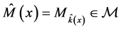

6. Specify a prior distribution for from the selected model.

7. Compute the posterior distribution for from the selected model.

8. Define a loss function.

9. Find the optimal decision rule. E.g. for square error loss, , or any quantity, e.g. posterior properties for.

More on Bayesian theory can be found in Gelman et al. [36] . When the analysis is conditioned on the ob- served data (conditional inference); there is no model selection uncertainty, only model uncertainty, since the data x (viewed as fixed) are used for all steps (including steps 3 and 4). However, if one needs the frequentist properties, the data should be viewed as random because steps 3 and 4 introduce model selection uncertainty and,. The difficulties are now similar those of frequentist model selection. The remaining uncertainty includes the choice of the statistical model, the prior, and the loss function.

3. Bayesian Post-Model-Selection Estimator

Bayesian post-model-selection estimator (BPMSE) is referred to the Bayes estimator obtained after a model selection procedure has been applied. Here, a squared error loss is considered, but the main idea remains unchanged for any other loss function. Given the selection procedure, BPMSE can been written as

(1)

where if model is selected and 0 otherwise. In the rest of the paper, for simplicity, each model will be replaced only by in the integrals.

Long-run performance of Bayes estimators: Usually, the goal of the analysis is to select a model for inference using any selection procedure. One is interested in evaluating the long run performance (frequentist performance) of the selected model. In general, Bayes estimators have good frequentist properties (e.g. Carlin and Louis [37] ; Bayarri and Berger [38] ). The Bayesian approach can also produce interval estimation with good performance, for example coverage probabilities. It is also known that if a Bayes estimator associated with a prior is unique, then it is admissible (Robert [31] ). There are also conditions under which Bayes estimator are minimax. The point is to see whether these frequentist properties still hold for Bayes estimators after model selection.

Interest is focused on studying the frequentist properties of. The difficulties here are similar to those encountered in frequentist PMSEs. This is due to the partition of the sample space X by the selection procedure. This makes it difficult to derive the coverage probability of confidence intervals.

The frequentist risk: The frequentist risk of BPMSEs is defined as

(2)

where L is a loss function. One can now see that this risk is difficult to compute; it is hard to prove admissibility and minimaxity properties of BPMSEs, since their associated priors are not known.

Coverage probabilities: When the data have been observed, one can construct a confidence region.

Suppose that after observing the data, model is selected. For large samples, Berger [39] considers the normal approximation

(3)

and then derives an approximate region at the level given by

where is the a-quantile of.

A stochastic version (assuming normality) is given by

The coverage probability of the stochastic form is given by

which is now difficult, as it involves computing the variance and expectation of BPMSE.

Consistency: Another frequentist property of Bayes estimators is consistency. It is shown that, under appropriate regularity conditions, Bayes estimators are consistent (Bayarri and Berger [38] ). A question is whether BPMSEs are consistent, but it is hard to prove because one does not know the priors associated with BPMSEs.

4. Adjusted Bayesian Model Averaging

In this framework, interest is focused with the long run performance of BPMSES, not on posterior evaluation, since in the posterior evaluation, the model selection uncertainty problem does not exist. Under model selection uncertainty, from Equation (1), a fundamental ingredient is the selection procedure S. This selection procedure should depend on the objective of the analyst and should be taken into account in modeling uncertainty at two levels: prior and posterior to the data analysis. In the following, we define the posterior quantity and derive Bayesian-post-model selection in a coherent way. The new method is referred to as Adjusted Bayesian model averaging (ABMA).

4.1. Prior Model Selection Uncertainty

The initial representation of model uncertainty is captured by parameter prior uncertainty and the model space prior, the selection procedure is used to update model prior. Formally, consider the possible models; assign a prior probability to the parameter of each model and a prior probability to each model with the data X viewed as random. Let be event model is selected, is considered to be the event model is true. The probability of this event is referred to as prior model selection probability of model and denoted by. This is to update prior model using the selection proce- dure S. may be informative or not, but is an informative prior. Making use of the fact that one of the models is true, can been computed as

(4)

where is the prior model selection probabilities of model given that is the true

model. is the probability that is actually selected given that it is really the true model.

The true state of the nature is that a given model is true; the decision here is to select a model. Given that model is true,. These probabilities can be computed as

(5)

The expectation is taken with respect to the true model, provided that these expectations exist. Note that these probabilities do not longer depend on the observed data.

Table 1 shows the true state of the world (nature) and the decision (the selected model). The , the probability that is selected, given that is the true model. Suppose that is the true model, one would like to be higher, ideally 1 (the correct decision). If model is not selected

with probability one, is called the probability of Type I error for model.

That is, if is the true model and the selection procedure S incorrectly does not select it, then the selection procedure has made a Type I Error.

On the other hand, if is the true model, but the selection procedure selects, then this selection procedure has made a Type II error, with probability,. The reliability of the selection criterion is given by the closeness of to 1.

4.2. Posterior Model Selection Uncertainty

When the data have been observed, the posterior model selection probability for each model is given by

(6)

Table 1. True state (M) and selected models ().

where

(7)

is the marginal likelihood of. For discrete, (7) is a summation. is the conditional probability that was the selected model. Computations are conditioned on each model, since one will never know the selection for random data. This is similar to the fact that the true model is not known, and each of the models can be viewed as a possible true model.

Posterior distribution: After the data x is observed, and given the selection procedure S, from the law of total probability, the posterior distribution of is then given by

(8)

is an average of the posterior of each model, , weighted by posterior model selection probability.

Posterior mean and variance:

Proposition 1 Under Equation (8), the posterior mean and variance are given by

(9)

where and are respectively the posterior mean and the posterior variance of for model if was the selected model.

Proof. Under Equation (8), the posterior mean is

The posterior variance under Equation (8) is

is the posterior expectation loss for model for taking the decision rule rather than.

The method can be then summarised as follows:

1. represents the prior model uncertainty,

2. updates prior model uncertainty by taking into account the selection procedure,

3. is the overall posterior representation of the model selection uncertainty.

Note that if the unconditional model selection probability is equal to model prior, then the proposed weights are the same as BMA weights, namely the probability that each model is true given the data,. For the proposed weights, one needs to compute the marginal likelihood and these model selection probabilities. Methods exist in the literature for doing such computations. These include Markov chain Monte Carlo methods, non-iterative Monte Carlo methods, and asymptotic methods. Other Bayesian methods based on mixtures include Ley and Steel [40] , Liang et al. [32] , Schäfer et al. [41] , Rodrguez and Walker [42] , and Abd and Al- Zaydi [43] . Some frequentist mixtures include Abd and Al-Zaydi [44] , and AL-Hussaini and Hussein [45] .

A basic property: From the non-negativity of Kullback-Leiber information divergence, it follows that:

(10)

where the expectation is taken with respect to the posterior distribution in Equation (8). This logarithm score rule was suggested by Good ( [46] ). This means that under the use of a selection criterion and the posterior distribution given in Equation (8), ABMA provides better predictive ability (under logarithm score rule) than any single selected model.

For computational purposes, can be written as

(11)

where is the Bayes factor, summarising the relative support for model versus model using posterior model selection probabilities. Using Laplace approximation of the marginal likekihood, the weights in Equation (11) become

(12)

where is Bayesian information criterion for model.

5. Applications

Let be a quantity of interest with prior and posterior (given data x); a sample space for any decision rule; a statistical model distribution of x. The frequentist risk of is

The Bayes risk of is and is constant.

For some models, beta prior will be used for; e.g beta prior as follows:, , then, therefore

is the Bayes estimate of. The marginal distribution of X is the beta-binomial, whose probability density function (Casella and Berger [47] ) is given by

Various results obtained in this Section are not sensitive to the variation of different parameters. R software [48] was used for computing.

5.1. Long Run Evaluation

5.1.1. Two-Model Choice

(a) and; with degenerate priors. Within the framework of hypothesis testing, Bernado and Smith [33] refer to (a) as “simple versus simple test” .

The posterior model probabilities are given by

.

Model 1 is selected if,

BMA corresponds to weighting the models with their posterior; the corresponding estimator is .

The BPMSE if is selected and otherwise.

For illustration of the case, we take, , , ,.

Figure 1 illustrates the performances of BPMSE, BMA and ABMA. BMA and ABMA have similar perfor- mances. Only points and are relevant since the true model is one of the two. However, for some regions of the parameter space, BMA does not perform better than BPMSE. It is clearly shown from Figure 1 that ABMA outperforms BPMSE and BMA.

Figure 2 shows these estimators all together, with smallest risk being ABMA for all regions of the parameter space; again ABMA outperforms BMA and BPMSE.

(b) Consider the following two models:, , noninformative prior and.

Let the selection procedure consisting of choosing the model with higher posterior.

and,

Figure 1. Risk of two proportions comparing BPMSE, BMA and ABMA estimators as a function of m.

Figure 2. Risk of two proportions comparing BPMSE, BMA and ABMA estimators as a function of m.

is chosen if.

.

.

and.

The parameters for simulating Figure 3 are, , that is,. Again, Figure 3 clearly shows that ABMA performs better than BPMSE and BMA.

(c) Consider the following two models:, (degenerate prior) and . Similar degenerate priors for model 1 can be seen in Robert [31] and Berger [39] .

Estimators for:

.

.

Figure 4 shows the MSE of BPMSE, BMA and ABMA. As can be seen BMA does not dominate BPMSE, but ABMA does. Figure 5 shows the MSE of BPMSE, BMA and ABMA. As can be seen BMA does not dominate BPMSE, but ABMA does.

5.1.2. Multi-Model Choice

(a) Consider also a choice between the following models: for arbitrary K models, with degenerate. Simulations shown in figure (fig:bma.30.simple.binomial.ps) are performed with and

(b) Consider also a choice between the following models: for arbitrary K models, , , , and.

Figure 6 shows the MSE of BPMSE, BMA and ABMA. As can be seen BMA does not dominate BPMSE, but ABMA does.

5.2. Evaluation with Integrated Risk

A good feature of integrated risk is that it allows a direct comparison of estimators (since it is a number). Con-

Figure 3. Risk of two proportions comparing BPMSE, BMA and ABMA as a function of m.

Figure 4. Risk of two proportions comparing BPMSE, BMA and ABMA as a function of m.

Figure 5. Risk of 30 simple models comparing BPMSE, BMA and ABMA as a function of m.

sider a choice between the following models: for arbitrary K models, , , ,.

For each model (between 10 and 200), the integrated risk is computed and comparisons of estimators is given in Figure 7. The ABMA dominates BPMSE, BMA does not. All Figures 1-7 presented here showed that the new method ABMA outperforms BMA and BPMSE in the sense of having smallest risk throughout the parameter space.

6. Concluding Remarks

This paper has proposed a new method of assigning weights for model averaging in a Bayesian approach when

Figure 6. Risk of 30 full models comparing BPMSE, BMA and ABMA as a function of m.

Figure 7. Integrated risks comparing BPMSE, BMA and ABMA as a func- tion of the number of models.

the frequentist properties of the estimator obtained after model selection are of interest. It was shown via Bernoulli trials that the new method performs better than Bayesian post-model selection and Bayesian model averaging estimators using risk function and integrated risk. The method needs to be applied in more realistic and myriads situations before it can be validated. In addition, further investigations are necessary to derive its theoretical properties, including large sample theory.

Acknowledgements

The authors thank the Editor and the referee for their comments on earlier versions of this paper.

Conflicts of Interest

The authors declare no conflicts of interest.

References

[1]	Clyde, M.A. and George, E.I. (2004) Model Uncertainty. Statistical Science, 19, 81-94. http://dx.doi.org/10.1214/088342304000000035
[2]	Hoeting, J.A., Madigan, D., Raftery, A.E. and Volinsky, C.T. (1999) Bayesian Model Averaging: A Tutorial (with Discussions). Statistical Science, 14, 382-417.
[3]	Marty, R., Fortin, V., Kuswanto, H., Favre, A.C. and Parent, E. (2015) Combining the Bayesian Processor of Output with Bayesian Model Averaging for Reliable Ensemble Forecasting. Journal of the Royal Statistical Society: Series C (Applied Statistics), 64, 75-92. http://dx.doi.org/10.1111/rssc.12062
[4]	Simmons, S.J., Chen, C., Li, X., Wang, Y., Piegorsch, W.W., Fang, Q., Hu, B. and Dunn, G.E. (2015) Bayesian Model Averaging for Benchmark Dose Estimation. Environmental and Ecological Statistics, 22, 5-16. http://dx.doi.org/10.1007/s10651-014-0285-4
[5]	Fan, T.H. and Wang, G.T. (2015) Bayesian Model Averaging in Longitudinal Regression Models with AR (1) Errors with Application to a Myopia Data Set. Journal of Statistical Computation and Simulation, 85, 1667-1678. http://dx.doi.org/10.1080/00949655.2014.891205
[6]	Corani, G. and Mignatti, A. (2015) Robust Bayesian Model Averaging for the Analysis of Presence—Absence Data. Environmental and Ecological Statistics, 22, 513-534. http://dx.doi.org/10.1007/s10651-014-0308-1
[7]	Tsiotas, G. (2015) A Quasi-Bayesian Model Averaging Approach for Conditional Quantile Models. Journal of Statistical Computation and Simulation, 85, 1963-1986. http://dx.doi.org/10.1080/00949655.2014.913044
[8]	Lenkoski, A., Eicher, T.S. and Raftery, A.E. (2014) Two-Stage Bayesian Model Averaging in Endogenous Variable Models. Econometric reviews, 33, 122-151. http://dx.doi.org/10.1080/07474938.2013.807150
[9]	Fan, T.H., Wang, G.T. and Yu, J.H. (2014) A New Algorithm in Bayesian Model Averaging in Regression Models. Communications in Statistics-Simulation and Computation, 43, 315-328. http://dx.doi.org/10.1080/03610918.2012.700750
[10]	Madadgar, S. and Moradkhani, H. (2014) Improved Bayesian Multimodeling: Integration of Copulas and Bayesian Model Averaging. Water Resources Research, 50, 9586-9603. http://dx.doi.org/10.1002/2014WR015965
[11]	Nguefack-Tsague, G. (2013) Bayesian Estimation of a Multivariate Mean under Model Uncertainty. International Journal of Mathematics and Statistics, 13, 83-92.
[12]	Koop, G., Leon-Gonzalez, R. and Strachan, R. (2012) Bayesian Model Averaging in the Instrumental Variable Regression Model. Journal of Econometrics, 171, 237-250. http://dx.doi.org/10.1016/j.jeconom.2012.06.005
[13]	Clyde, M.A. and Iversen, E.S. (2015) Bayesian Model Averaging in the M-Open Framework. In: Bayesian Theory and Applications, 483-498. Oxford University Press, Oxford.
[14]	Berk, R., Brown, L., Buja, A., Zhang, K. and Zhao, I. (2013) Valid Post-Selection Inference. Annals of Statistics, 41, 802-837. http://dx.doi.org/10.1214/12-AOS1077
[15]	Leeb, H. and P?tscher, B.M. (2009) Model Selection. In: Handbook of financial time series, 889-925. Springer Berlin Heidelberg. http://dx.doi.org/10.1007/978-3-540-71297-8_39
[16]	Burnham, K.P. and Anderson, D.R. (2013) Model Selection and Multimodel Inference: A Practical Information-Theo- retic Approach. Springer, Cambridge.
[17]	Nguefack-Tsague, G. (2013) An Alternative Derivation of Some Commons Distributions Functions: A Post-Model Selection Approach. International Journal of Applied Mathematics and Statistics, 42, 138-147.
[18]	Nguefack-Tsague, G. (2013) On Bootstrap and Post-Model Selection Inference. International Journal of Mathematics and Computation, 21, 51-64.
[19]	Nguefack-Tsague, G. (2014) Estimation of a Multivariate Mean under Model Selection Uncertainty. Pakistan Journal of Statistics and Operation Research, 10, 131-145. http://dx.doi.org/10.18187/pjsor.v10i1.449
[20]	Nguefack-Tsague, G. (2014) On Optimal Weighting Scheme in Model Averaging. American Journal of Applied Mathematics and Statistics, 2, 150-156. http://dx.doi.org/10.12691/ajams-2-3-9
[21]	Zucchini, W., Claeskens, G. and Nguefack-Tsague, G. (2011) Model Selection. In: Lovric, M., Ed., International Encyclopedia of Statistical Science, Springer, Berlin, 830-833. http://dx.doi.org/10.1007/978-3-642-04898-2_373
[22]	Nguefack-Tsague, G. and Zucchini, W. (2011) Post-Model Selection Inference and Model Averaging. Pakistan Journal of Statistics and Operation Research, 7, 347-361. http://dx.doi.org/10.18187/pjsor.v7i2-Sp.292
[23]	Zucchini, W. (2000) An Introduction to Model Selection. Journal of Mathematical Psychology, 44, 41-61. http://dx.doi.org/10.1006/jmps.1999.1276
[24]	Schwarz, G. (1978) Estimating the Dimension of a Model. Annals of Statistics, 6, 461-464. http://dx.doi.org/10.1214/aos/1176344136
[25]	Guan, Y. and Stephens, M. (2011) Bayesian Variable Selection Regression for Genome-Wide Association Studies, and Other Large-Scale Problems. Annals of Applied Statistics, 5, 1780-1815. http://dx.doi.org/10.1214/11-AOAS455
[26]	Clyde, M.A., Ghosh, J. and Littman, M.L. (2011) Bayesian Adaptive Sampling for Variable Selection and Model Averaging. Journal of Computational and Graphical Statistics, 20, 80-101. http://dx.doi.org/10.1198/jcgs.2010.09049
[27]	Clyde, M.A. (1999) Bayesian Model Averaging and Model Search Strategies. In: Bayesian Statistics 6: Proceedings of the 6th Valencia International Meetin, Oxford University Press, Oxford, 157-188.
[28]	Nguefack-Tsague, G. (2011) Using Bayesian Networks to Model Hierarchical Relationships in Epidemiological Studies. Epidemiology and Health, 33, Article ID: e2011006. http://dx.doi.org/10.4178/epih/e2011006
[29]	Carvalho, C.M. and Scott, J.G. (2009) Objective Bayesian Model Selection in Gaussian Graphical Models. Biometrika, 96, 497-515. http://dx.doi.org/10.1093/biomet/asp017
[30]	Fridley, B.L. (2009) Bayesian Variable and Model Selection Methods for Genetic Association Studies. Genetic Epidemiology, 33, 27-37. http://dx.doi.org/10.1002/gepi.20353
[31]	Robert, C.P. (2007) Bayesian Choice: From Decision-Theoretic Foundations to Computational Implementation. Springer, New York.
[32]	Liang, F., Paulo, R., Molina, G., Clyde, M.A. and Berger, J.O. (2008) Mixtures of g Priors for Bayesian Variable Selection. Journal of the American Statistical Association, 103, 174-200. http://dx.doi.org/10.1198/016214507000001337
[33]	Bernado, J.M. and Smith, A.F.M. (1994) Bayesian Theory. Wiley, New York. http://dx.doi.org/10.1002/9780470316870
[34]	Nguefack-Tsague, G. and Ingo, B. (2014) A Focused Bayesian Information Criterion. Advances in Statistics, 2014, Article ID: 504325. http://dx.doi.org/10.1155/2014/504325
[35]	Nguefack-Tsague, G. and Zucchini, W. (2016) A Mixture-Based Bayesian Model Averaging Method. Open Journal of Statistics, 6, 220-228. http://dx.doi.org/10.4236/ojs.2016.62019
[36]	Gelman, A., Carlin, J.B., Stern, H.S. and Rubin, D.B. (2014) Bayesian Data Analysis. Chapman and Hall/CRC, London.
[37]	Carlin, B.P. and Louis, T.A. (2000) Bayes and Empirical Bayes Methods for Data Analysis. Chapman and Hall, London. http://dx.doi.org/10.1201/9781420057669
[38]	Bayarri, M.J. and Berger, J.O. (2004) The Interplay of Bayesian and Frequentist Analysis. Statistical Science, 19, 58- 80. http://dx.doi.org/10.1214/088342304000000116
[39]	Berger, J. (1985) Statistical Decision Theory and Bayesian Analysis. Springer, New York. http://dx.doi.org/10.1007/978-1-4757-4286-2
[40]	Ley, E. and Steel, M.F.J. (2012) Mixtures of g-Priors for Bayesian Model Averaging with Economic Applications. Journal of Econometrics, 171, 251-266. http://dx.doi.org/10.1016/j.jeconom.2012.06.009
[41]	Sch?fer, M.Y., Radon, T., Klein, S., Herrmann, H., Schwender, P., Verveer, J. and Ickstadt, K. (2015) A Bayesian Mixture Model to Quantify Parameters of Spatial Clustering. Computational Statistics and Data Analysis, 92, 163-176. http://dx.doi.org/10.1016/j.csda.2015.07.004
[42]	Rodrguez, C.E. and Walker, S.G. (2014) Univariate Bayesian Nonparametric Mixture Modeling with Unimodal Kernels. Statistics and Computing, 24, 35-49. http://dx.doi.org/10.1007/s11222-012-9351-7
[43]	Abd, E.B.A. and Al-Zaydi, A.M. (2015) Bayesian Prediction of Future Generalized Order Statistics from a Class of Finite Mixture Distributions. Open Journal of Statistics, 5, 585-599. http://dx.doi.org/10.4236/ojs.2015.56060
[44]	Abd, E.B.A. and Al-Zaydi, A.M. (2013) Inferences under a Class of Finite Mixture Distributions Based on Generalized Order Statistics. Open Journal of Statistics, 3, 231-244. http://dx.doi.org/10.4236/ojs.2013.34027
[45]	AL-Hussaini, E.K. and Hussein, M. (2012) Estimation under a Finite Mixture of Exponentiated Exponential Components Model and Balanced Square Error loss. Open Journal of Statistics, 2, 28-38. http://dx.doi.org/10.4236/ojs.2012.21004
[46]	Good, I.J. (1952) Rational Decisions. Journal of the Royal Statistical Society, Series B, 14, 107-114.
[47]	Casella, G. and Berger, R.L. (2001) Statistical Inference. Wadsworth and Brooks/Cole, California.
[48]	R Development Core Team (2015) R: A Language and Environment for Statistical Computing. R Foundation for Statistical Computing, Vienna.