Resolution of Relationship between Organizational Performance and Human Resource Management through Nonlinear Modeling ()
Received 8 October 2015; accepted 25 December 2015; published 28 December 2015

1. Introduction
Human Resource Management (HRM) is a critical input in enhancing the business results. FIRM criteria cover the planning, managing and improving the Human Resources; identifying, developing and sustaining people’s knowledge and competencies; involving and empowering people. All these factors have an effect on business results, because Human Resources are key assets. HRM has a significant impact on the performance of the manufacturing business (firm).
The relation between the HRM and the firm performance is analyzed statistically by many researchers in the literature. However there are very few nonlinear approaches in literature for finding the relation between Human Resource Management (FIRM) and firm performance. One method for this nonlinear approach may be Artificial Neural Networks (ANN’s). Artificial Neural Networks (ANN’s) are systems that are deliberately constructed to make use of some organizational principles resembling those of the human brain. Generally speaking, artificial neural networks are computing systems made up of a number of simple highly interconnected signal or information processing units that are called as artificial neurons [1] -[4] . This model can be used in many different problem solutions including nonlinear modeling. Hence we decided to use one of the modeling techniques of ANN approach which is called as Radial Basis Function (RBF) in Human Resource Management. In this thesis our aim is to check whether there is a nonlinear relation between the Human Resource Management and the firm performance with the help of the Artificial Neural Network (ANN) modeling technique.
In Section 2, we presented the modeling technique called Artificial Neural Networks. We introduced the history of ANN, how they operate and their analogy to the brain. In the same chapter, we explained one of the modeling techniques used in ANN that is called as Radial Basis Function (RBF) networks. We used this modeling technique for finding the relation between the Human Resource Management and firm performance.
In the following section, Section 2.4, we introduced the Human Resource Management. We explained the importance of HRM and gave the background of it. Also we mentioned some of the international studies about the relation between Human Resource Management and Firm Performance.
The experimental design and collected results are given in Section 3. In this last section of this research, the explanations of the 21 parameters (12 input parameters + 9 output parameters) used for finding the relation between the Human Resource Management and the firm performance are explained. The experimental results are shown with the help of tables and figures. The deductions, conclusions and observations are given briefly in the conclusion section.
2. Artificial Neural Networks
Artificial Neural Networks are relatively crude electronic models based on the neural structure of the brain. The brain basically learns from experience. It is natural proof that some problems that are beyond the scope of current computers are indeed solvable by small energy efficient packages. This brain modeling also promises a less technical way to develop machine solutions. This new approach to computing also provides a more graceful degradation during system overload than its more traditional counterparts.
2.1. Radial Basis Function (RBF)
The One of the interesting type of Artificial Neural Networks, Radial-Basis Function (RBF) networks, was first introduced by M. J. D. Powell in 1985. This type of Neural Network design can be viewed as a curve-fitting (approximation) problem in high-dimensional space. According to this viewpoint, learning is equivalent to finding a surface in hyperspace that provides the best fits to the training data. The “best fit” is measured in some statistical sense. RBF in its most basic form consists of 3 layers, with one hidden layer. Here, the hidden units provide a set of “functions” that constitutes an arbitrary “basis” for input patterns, and these functions are called radial-basis functions. One of the misconceptions surrounding the value unit architecture is based upon its use of a Gaussian activation function. This is because another network architecture, the Radial Basis Function (RBF) network uses a similar activation function. That, however, is where the similarities end. The RBF network is a three-layer feed forward network that uses a linear transfer function for the output units and a nonlinear transfer function (normally the Gaussian) for the hidden units. The input layer simply consists of 71 units connected by weighted connections to the hidden layer and a possible smoothing factor matrix. A hidden unit can be described as representing a point x in n-dimensional pattern space. Consequently the net input to a hidden unit is a distance measure between some input, xi, presented at the input layer and the point represented by the hidden unit; that is. This means that the net input to a unit is a monotonic function as opposed to the nonmonotonic activation function of the value unit. The Gaussian is then applied to the net input to produce a radial function of the distance between each pattern vector and each hidden unit weight vector. Hence, a RBF unit carves a hyper sphere within a pattern space whereas a value unit carves a hyper bar.
In general, an RBF network can be described as constructing global approximations to functions using combinations of basic functions centered around weight vectors. In fact, it has been shown that RBF networks are universal function approximators. Practically, however, the approximated function must be smooth and piecewise continuous. Consequently, although RBF networks can be used for discrimination and classification tasks, binary pattern classification functions that are not piecewise continuous (e.g., parity) pose problems for RBF networks Thus, RB The RBF network used in this work is given in Figure 1. It consists of an input layer, one hidden layer and an output layer.
The transformation from input space to output is nonlinear and the transformation from hidden unit space to output space is linear, the set of Basis functions  is defined as follows
 (1)
(1)
where  are the set of M centers to be determined and x is one of the training (input) data in a set
  of size N. Typically, the number of basis functions, M is less than the number of data points. Our aim is to find the suitable w values in order to minimize the Euclidean Norm.
 , where
  (2)
(2)
 (3)
(3)
 .
.
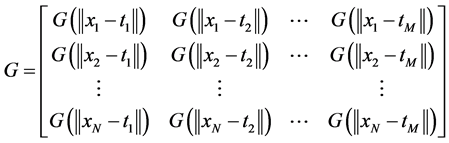
The vector d is an N-dimensional desired response vector, the matrix G is an N ´ M matrix of Green’s function and the vector w is M-by-1 weight vector for the linear transformation from hidden unit space to output space. The minimum norm solution to the over determined least squares data fitting problem can be given as follows
 (4)
(4)
Formula 2.3
The set of centers  can be selected randomly from the set of data points, can be selected
using the clustering techniques to find the suitable centers or can be selected using gradient descent algorithm. In this study, we used random selection to find the set of centers for the Radial Basis Functions.
2.2. Human Resource Management (HRM)
In last 10 year research has been made to search and establish link between human resources applications and firm performance. Competitive global economy is increasing very fast and making the firms to use all of their resources as a competitive advantage. Recently human resources have been accepted as one of the most important resources for competition. These phenomena increased the vision of Strategic Human Resource Management. Firm Performance is the general organizational aim, so research about strategic human resources management is diverted to the understanding of relationship between human resources and firm performance. General idea of these researches is that if firms are using best selection system, training program or reward system these firms will have very important advantage for competition compared to other firms. Researches are indicating that there are links between human resources management applications and many performance measures [5] -[7] .
Of all the advances in management thinking which transpired during the twentieth century, perhaps none has been so important as those that have occurred within the domain of what we now call human resource management. These advances have come in two basic forms. First, it has been learned that all business organizations (indeed, all organizations of any purpose) depend on their people for success. Second, it has been learned that by proper coordination, the people of an organization can achieve more by working together as a team than they can by working singly. The development of concepts such as the learning organization, human capital and knowledge capital are the building blocks of the new styles of organization now emerging. The coming of age of the employment management movement can be said to be marked by the publication of a special edition of the Annals of the American Academy of Political and Social Science in May 1916. We have only been able to reprint a small selection of articles here, but the issue was co-edited by Bloomfield and the opening articles were by Ernest Nichols, President of Dartmouth College and intimately connected with the early moves to train employment managers, and by William Redfield, US Secretary of Commerce in the Wilson administration and a strong supporter of the movement. Redfield in particular hammers home the point that if an organization’s people are as important as its machines, then they deserve the same care. The following five years saw a flood of literature on this new discipline, much of it extraordinarily good and forward-thinking. Of general interest in this collection are Frankel and Fleischer’s The Human Factor in Industiy (1920), in my opinion the best single textbook on the subject, and also the selections from Tead and Metcalf s Personnel Administration (1920). Ordway Tead was a guru of some note on this subject, and his views can be considered as representative of the profession at the time; his work was still being cited twenty years later by Lyndall Urwick. Other valuable pieces include Douglas’s article’ Plant Administration of Labor’ from the Journal of Political Economy (1919), Kennedy’s “Employment Management and Industrial Relations” from Industrial Management (1919) and Voorhees’s “Human Nature and Personnel Management”, also from Industrial Management (1920). Two useful critiques of employment management are Richardson (1919) and Fish (1920), both from Industrial Management. All these articles make a number of points, notably that employment management/personnel management cannot succeed unless it has the backing of top management and is considered a principle executive function [7] [8] .
The bubble economy decade, where for many companies profits and growth were assured despite the competence (or incompetence) of management, effectively masked the growing malaise of Asian organizations. The signs were there, as a review of the past items on the Chao Phraya River Rat would attest. Over five years, the Rat’s column drew attention to monstrous staff turnover rates, which meant that any investment in development or training was to naught anyway, as staffs were likely to leave any time for a job which paid a few dollars extra, and often in an industry or function totally unrelated. We referred to the unsustainability of professional and management salaries, and salary packages and perquisites so over valued and out-of-kilter with other economies that warning bells about an Asian crisis should have re sounded well before that fateful day in June [9] [10] .
In the meantime, interest in MBA and professional qualifications was increasing, and appealed to many for the prestige and authority they bestowed on the holder. However, these qualifications rarely integrated well with individual and organizational career and skills development, and were valued as status symbols rather than an experience that “added value” to the real worth of an individual to an organization. The race for the MBA merely added costs to a company’s payroll (in having to pay extra for the perceived value of an MBA, or sponsoring studies) with limited real benefit to the bottom line [11] [12] .
3. Experimental Analysis and Results
In this research, our aim is to establish a relationship between the Human Resource Management and the organizational performance using Artificial Neural Networks. 21 parameters were obtained from 54 companies in Turkey to achieve this goal. From these 21 parameters, 12 of them were used as input parameters and the rest were used as output parameters. These parameters can be explained briefly as follows:
Input Parameters
1) IDO (Turnover rate): the ratio of the number of workers that had to be replaced in a given time period to total number of workers. This rate can be calculated by dividing the number of workers that left the company to total number of workers.
2) DEV (Absence Rate): is a rate that measures the absence of workers depend on day. This rate can be calculated by dividing total absence of workers in year to total working days (average number of workers in a year*total working days of that year) of same year.
3) KBIK1V1 (HRM cost per capita): HRM cost means total expenses of the personnel that work in Human Resource Management department. This cost also includes hardware, software and other equipment expenses that are used by HRM department. This cost can be calculated by dividing the total expenses of HRM department to the number of full time workers of company.
4) IKMBO: This rate gives the percentage of HRM expenses in total personnel expenses and can be calculated for any period by dividing HRM cost to total personnel cost.
5) IICMTMO: This rate gives the percentage of HRM expenses in total expenses and can be calculated for any period by dividing HRM cost to total firm expenses.
6) TPMTMO: One of the most important cost for firms is Personnel cost. This rate can be calculated by dividing total personnel expenses to total firm expenses and shows the percentage of personnel expense in total firm expenses.
7) KBEGM (Education Expenses Per Capital): Training applications are very important for firm success and competition. Many search shows that if any firm is giving importance and making investment about training these type of firms are being more successful compared to others. This value can be calculated by dividing total training expenses of any year to total number of worker.
8) EGITSAATM: average training time that is given to each worker in M category during one year.
9) EGITSAATB: average training time that is given to each worker in B category during one year.
10) IKFI: Related with measuring human resources planning, hiring, selection, training, price management etc. There are many measures to analyze IKFI.
11) IICPGFAK1: First input parameter found by factor analyzing (using SPSS) of the answers given about Human Resources perceptional measures.
12) IKPGFAIC2: Second input parameter found by factor analyzing (using SPSS) of the answers given about Human Resources perceptional measures.
Output Parameters
1) IV (Labor productivity): Productivity and Unit Wage Costs are key economic indicators used to measure the efficiency and competitiveness of the economy. They are constructed as ratios of other indicators and are published as indices. Two measures of productivity are produced: Output per filled job and Output per hour worked.
2) KO (Profitability ratio): The analysis of a company’s earnings tells the investor how well management is using the company’s resources. Gross profit margin, operating profit margin and net profit margin ratios are useful for internal trend lines and external comparisons; especially in industries such as food products and cosmetics where turnover is high and competition severe. The gross profit margin is an indication of management’s efficiency in turning over the company’s goods to a profit. It shows the company’s rate of profit after allowing for the cost of goods sold.
3) YGDO: (Rate of return): The internal rate of return (IRR) method of analyzing a major purchase or project allows you to consider the time value of money. It allows you to find the interest rate that is equivalent to the dollar returns you expect from your project. Once you know the rate, you can compare it to the rates you could earn by investing your money in other projects or investments. If the internal rate of return is less than the cost of borrowing used to fund your project, the project will clearly be a money-loser. However, usually a business owner will insist that in order to be acceptable, a project must be expected to earn an IRR that is at least several percentage points higher than the cost of borrowing, to compensate the company for its risk, time, and trouble associated with the project.
4) VGDO (Rate of asset): A rate of resource that is controlled by an enterprise as a result of past events and from which future economic benefits are expected to flow to the enterprise.
5) KBK (profit per worker): In firms workforce is also important like capital so profit from each worker is a measure that shows the profitability of a firm.
6) SGDO (capital rate): If you’re going to invest (whether it’s in stocks, real estate or even rare stamps), you have to realize capital gains. After all, whether you win or lose with your picks.
The determination of the cost of capital rate consists of four distinct steps:
a) Determination of net rail investment,
b) Determination of capital structure,
c) Determination of the cost rates for each component of the capital structure which includes the cost of common equity rate and,
d) Calculation of the weighted average cost of capital rate, which includes an allowance for income tax.
7) TVO: This measure can be found by dividing total assets of firm into number of workers.
8) FPGFAK1: First output parameter found by factor analyzing (using SPSS) of the answers given about firm perceptional performance measures.
9) FPGFAK2: Second output parameter found by factor analyzing (using SPSS) of the answers given about firm perceptional performance measures.
For 54 companies in Turkey, these 21 parameters are collected for the years 2000 and 2001. Hence we have all together 108 data set (54*2) consisting of these 21 parameters. Among these 54 companies, 10 of them are randomly selected as testing data and the rest were used as training data. Hence we have 20 testing data set and 88 training data set. These 21 parameters are normalized according to the formulas given below:
1) IDO = IDO/20
2) DEV = DEV/10
3) KBIKM = log10 (KBIKM +1)
4) IKMBO = log10 (IKMB0 + 1)
5) IKMTMO = IKMTMO/10
6) TPMTMO = logl0 (TPMTMO)
7) KBEGM = log10 (KBEGM + 1)
8) EGITSAATM = EGITSAATM/60
9) EGITSAATB = EGITSAATB/60
10) HUI = logl0 (IKFI)
11) IKPGFAK1 = (IKPGFAKI + 3)/4
12) IKPGFAK2 = (IKPGFAK2 + 3)/5
13) IV = logl0 (IV)
14) KO = logl0 (K0 + 26)
15) YGDO = logl0 (YGDO + 32)
16) VGDO = logl0 (VGDO + 21)
17) KBK = logl0 (KBK + 6000)
18) SGDO = log10 (SGDO)
19) TVO logl0 (TVO)
20) FPGFAK1 = (FPGFAK1 + 3)/5
21) FPGFAK2 = (FPGFAK2 + 3)/5
The reason of normalizing the parameters is that to equate the effects of these parameters in the model and to match with the model requirements. First of all, we observed all the relations between the actual input parameters and the actual output parameters.
The reason of normalizing the parameters is that to equate the effects of these parameters in the model and to match with the model requirements. First of all, we observed all the relations between the actual input parameters and the actual output parameters. In Figures 2-4, we plotted only three of these relations.
From Figure 2, it is clear that there is no relation between the input parameter (IDO) and the output parameter
![]()
Figure 2. Actual output (FPGFAK2) parameters with respect to actual input (IDO) parameters (only the first 20 are plotted).
![]()
Figure 3. Actual output (IV) parameters with respect to actual input (DEV) parameters (only the first 20 are plotted).
![]()
Figure 4. Actual output (TVO) parameters with respect to actual input (KBIKM) parameters (only the first 20 are plotted).
(FPGFAK2). In Figure 3, the relation obtained between the input parameter (DEV) and the output parameter (IV) shows that this relation can be linearized. However the result that we obtained between the input parameter (KBIKM) and the output parameter (TVO) in Figure 4 shows that not all the relations can be linearized. Hence we decided to find the general relation between the input and the output parameters through the use of RBF network.
As we mentioned in Section 2, we selected the centers of the Radial Basis Functions randomly, but the number of the centers are not decided. To decide what will be the suitable number of centers in this study, we obtained the total training error between the actual output and the experimental result, for the 9 output parameters by using the number of the centers as (5, 6, 7, 8, 10, 12, 14, 16). The training error is an Euclidean distance between the 88 actual output parameters and the outputs obtained through the use of nonlinear model. The results obtained for the two outputs are shown in Figure 5 and Figure 6. From these figures we observed that 8 centers are enough to represent the relation that we are looking for. Hence from this point on, all the results are obtained by fixing the number of centers to eight.
After training the model by fixing the number of centers to eight, our first observation is to check whether the actual (real) training data matches with the experimental output or not. To do this we plotted the best 10 matches between the actual training data (Real Outputs) and experimental results (Program Outputs) for all 9 output parameters using different figures for each output parameters. We also gave the total Euclidean error obtained for the 88 training data. These results are given in Figures 7-14.
From these figures what we observed is that the actual outputs and the experimental outputs closely match. Also from the total training error we can easily say that the deviation between the actual output and program output is not very big. Hence we can conclude that our model learned the relation between the 12 input parameters and 9 output parameters.
The next step in this thesis is to find how well the actual output and experimental output matches for the testing data. This is very important since it shows us how well the model suited to this nonlinear relation. First of all we tabulated the Euclidean error between the actual outputs for all 20 testing data in Table 1.
The Euclidean distance given above is calculated by finding the distance between the 9 actual output and 9 experimental outputs for each testing data. The results showed that even for testing data the error is not significant. From this table, we selected the best 5 results (test data: 4, 7, 13, 14, 16) and plotted them in Figures 15-19.
![]()
Figure 5. Total training error as the number of centers are changing for TVO output parameter.
![]()
Figure 6. Total training error as the number of centers are changing for FPGFAK2 output parameter.
![]()
Figure 7. Real output and program output for training data for the IV output parameter (total training error: 5,44228).
![]()
Figure 8. Real output and program output for training data for the KO output parameter (total training error: 2,050884).
![]()
Figure 9. Real output and program output for training data for the YGD output parameter (total training error: 2,438809).
![]()
Figure 10. Real output and program output for training data for the VGD output parameter (total training error: 1,838303).
![]()
Figure 11. Real output and program output for training data for the KBK output parameter (total training error: 3,490306).
![]()
Figure 12. Real output and program output for training data for the SGDO output parameter (total training error: 6,346784).
![]()
Figure 13. Real output and program output for training data for the TVO output parameter (total training error: 3,562598).
![]()
Figure 14. Real output and program output for training data for the FPGFAK2 output parameter (total training error: 2,048678).
![]()
Figure 15. Actual output and experimental output for the 4’th testing data.
![]()
Table 1. Researchers conducted on relationship between HRM and organizational performance.
![]()
Figure 16. Actual output and experimental output for the 7’th testing data.
From these figures our detection is that the nonlinear model that we used represents the general behavior of the companies corresponding to the selected parameters.
4. Conclusion
In the last decade, many researches have been made to find a relation between the Human Resources and Firm Performance. Many of these studies are conducted on the basis of statistical approaches and find the correlation between the parameters. In all these applications the main criteria to be checked are weather the parameters at
![]()
Figure 17. Actual output and experimental output for the 13’th testing data.
![]()
Figure 18. Actual output and experimental output for the 14’th testing data.
![]()
Figure 19. Actual output and experimental output for the 16’th testing data.
hand are linearly related with each other or not.
In this research, our aim was to find whether the relation between the Human Resources and Firm Performance can be modeled nonlinearly or not. To check this claim we used one of the modeling techniques, namely the Radial Basis Function. This technique is one of the approaches used in Artificial Neural Networks for representing any kind of relation. From our experimental results, our conclusion can be summarized as follows.
When the output parameters are plotted with respect to input parameters, the relation observed for both actual and experimental data shows that the relation is not linear and may be linearized for some of these relations but not for all. In general hence our suggestion is to use nonlinear relation (model) between the input and output parameters.
By using the Radial Basis Functions in the modeling of this nonlinear relation, we observed that nonlinear model is capable of representing the relation at hand.
To check the performance of our model we used the 20 data sets obtained from 10 companies. This data set was not used in the training phase. We plotted both the actual and experimental outputs for the 5 best fitted data sets and gave the Euclidian errors for all 20 data sets. From these results, we conclude that the relation between the input and output parameters can be modeled nonlinearly.
As a future work, we suggest using different kind of nonlinear models for representing the relation between the Human Resource Management and Firm Performance and combine their results in such way that the error between the actual output parameters and the experimental output parameters will be minimized. Also the number of training and testing data can be increased to make this work more general.