Boundedness and Oscillation of Third Order Neutral Differential Equations with Deviating Arguments

Elmetwally M. Elabbasy^*, Magdy Y. Barsoum, Osama Moaaz

Department of Mathematics, Faculty of Science, Mansoura University, Mansoura, Egypt.

DOI: 10.4236/jamp.2015.311164                

Abstract

we consider the third-order neutral functional differential equations with deviating arguments. A new theorem is presented that improves a number of results reported in the literature. Examples are included to illustrate new results.

Keywords

Oscillation, Third Order, Neutral Delay Differential Equations

1. Introduction

In this paper we consider third order neutral differential equations of the form

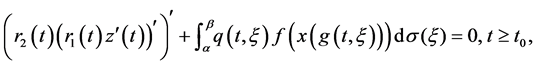(1)

where 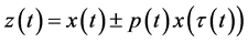and the following conditions are satisfied

(A₁) 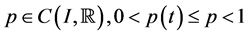and,

(A₂)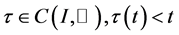, is strictly increasing, and we define

(A₃)

(A₄), f is non-decreasing and for,

(A₅) and is not zero on any half line

(A₆), for and, is continuous, has positive partial derivative on with respect to t, nondecreasing with respect to and

(A₇), is nondecreasing and the integral of Equation (1) is in the sense Riemann-stieltijes.

We mean by a solution of Equation (1) a function, such that, ,

and exist and are continuous on. A nontrivial solution of (1) is called oscillatory if it has arbitrarily large zeros, otherwise it is called non-oscillatory.

Asymptotic properties of solutions of differential equations of the second and third order have been subject of intensive studying in the literature. This problem for neutral differential equations has received considerable attention in recent years (see [1] - [11] ).

Recently, in [12] by using Riccati technique, have established some general oscillation criteria for third-order neutral differential equation

In [3] , Candan presented several oscillation criteria for third order neutral delay differential equation

[9] and [13] obtained some oscillation criteria for study third order nonlinear neutral differential equations

and

In this paper, we establish some oscillation criteria for Equation (1), which complement and extend the results in [3] [13] .

We begin with analyzing of the asymptotic behavior of possible non-oscillatory solutions of the Equation (1) in the case when. Let be a non-oscillatory solution of (1) on. From (1) it follows that the function has to be eventually of constant sign, so either

(a)

or

(b)

for all sufficiently large t. Denote by [or] the set of all non-oscillatory solutions of the Equation (1) such that (a) [or (b)] is satisfied. We begin with some useful lemmas.

Lemma 1.1 Let. Assume that (A₁) and (A₂) hold and x be continuous non-oscillatory solution of the functional inequality (a). Then

Lemma 1.2 Let. Assume that (A₁) and (A₂) hold and x be continuous non-oscillatory solution of the functional inequality (b). If then

These lemmas are modifications of the Lemma 1 in the paper [14] and the Lemma 2 in the paper [13] .

2. Main Results

In this part, for the sake of convenience, we introduce the following notation:

2.1. Oscillation Criteria If

In this section, we will establish some oscillation criteria for Equation (1) in the case when and.

Lemma 2.1 Let x be a bounded positive solution of Equation (1) on the interval I. Then there exists a such that has the following properties:

(2)

Proof. Let x be a bounded positive solution of Equation (1) on the interval I. From (A₁), (A₂) and (A₆), there exists a such that, and for. Then is bounded and non-oscillatory. Thus, Equation (1) implies that

Hence, the function is a non-increasing and of one sign. We claim that for. Suppose that for. Then there exists a and constant such that

By integrating the last inequality from to t, we get

Letting, from (A₃), we have. Then there exists a and constant such that

By integrating this inequality from to t and using (A₃), we get. This yields that and this contradicts the Lemma 1.1. Now we have for. Hence is increasing function and we have two possible cases for either eventually or

eventually for. If for, then there exist a and a constant such that

By integrating this inequality from to t and using (A₃), we get. This means that and we get for all sufficiently large t. Then, which contradicts the boundedness of. Hence, for.

Theorem 2.1 if

(3)

Then every bounded solution of Equation (1) is either oscillatory or tends to zero.

Proof. Let x be a bounded non-oscillatory solution of Equation (1) on the interval I. Without loss of generality we may assume that. From Lemma 2.1, we get that (2) holds. New, we have

for all sufficiently large t. Repeating this procedure and the monotonicity of, we obtain that there exists an

integer such that and

where. Hence, we get

(4)

Thus, from Equation (1), we obtain

(5)

Now, since is bounded decreasing function, then there exist such that

If for, then and which contradicts the Lemma 1.1. Therefore for and. We shall prove that. Let. For, we obtain

Thus, form Lemma 2.1, we get

(6)

So, for, we have

Hence, from (6), we get

(7)

where. Let us define function

We note that. Deriving partially with respect to s and using Lemma 2.1, (A₄) and (A₆), we get

From (5), we have. Hence, we obtain

(8)

By (A₄) and (A₆), we get

Thus, from (7), we have

(9)

Then, substituting (8) in (9), it follows that

By integrating this inequality from to t with respect to s, we obtain

(10)

where. Since, we get

Hence, from (10), we have

which contradicts (3). Therefore, and according to the Lemma 1.2 we have that.

In the following Theorem, we establish some sufficient conditions for boundedness and oscillation of Equation (1) under the condition

(11)

Theorem 2.2 Let (11) holds. If there exist an integer such that

(12)

then every bounded solution of Equation (1) is oscillatory.

Proof. Let x be a bounded non-oscillatory solution of Equation (1) on the interval I. Without loss of generality we may assume that. We can proceed exactly as in the proof of Theorem 2.1 and we use the fact that (12) implies (3). Hence, we get a non-oscillatory solution with the properties, ,

and for, and. New, from (4), there exists such that

Thus, Equation (1) implies that

By integrating this inequality from to t, we get

where. Thus, we obtain

(13)

where. Since, from the Inequality (7), we get

(14)

Combining (13) and (14), we have

Hence, we get

for and this contradicts the condition (12).

Corollary 2.1 Let (11) holds. If

(15)

then every bounded solution of Equation (1) is oscillatory.

Example 2.1 Consider the differential equation

where. We have

and. Thus, all conditions of Corollary 2.1 are satisfied then all bounded solutions

of the above equation are oscillatory.

Remark 2.1 If and then, our results extend the results in [13] .

2.2. Oscillation Criteria If

In this section, we will present some oscillation criteria for Equation (1) under the case and the condition

(16)

Lemma 2.2 If is an eventually positive solution of (1), then for sufficiently large t, there are only two possible cases:

(i)

(ii)

Proof. The proof of this lemma is similar to the proof Lemma 1 in [9] and we omit the details.

Theorem 2.3 Let (16) holds. If

(17)

and there exist a positive real function such that

(18)

Then every solution of Equation (1) is either oscillatory or tends to zero.

Proof. Let x be a non-oscillatory solution of Equation (1) on the interval I. Without loss of generality we may assume that. Then there exists a such that, and for. By Lemma 2.2, we have two cases for. In the Case (i), since and, we get

. Let, then we have for all and t enough large. Choosing, we obtain

where. Hence, from (1), (A₆) and (16), we have

By integrating two times from t to, we get

Integrating the last inequality from to, we obtain

This contradicts to the condition (17), then, which implies that. In the Case (ii),

since and. Then there exist a such that

for. Thus, from (1), (A₄) and (A₆), we get

(19)

Also, we have

Since, we obtain

(20)

Now, we define

By differentiating and using (19) and (20), we get

Hence, we obtain

By integrating the above inequality from to t we have

Taking the superior limit as and using (18), we get which contradicts that. This completes the proof of Theorem 2.3.

Remark 2.2 We can rewrite the condition (17) in the Theorem 2.3 as following

Remark 2.3 If and, then our results extend the results in [3] .

Example 2.2 Consider the differential equation

where and. Choosing and. Thus, all conditions of Theorem 2.3

are satisfied then every solutions of this equation is either oscillatory or tends to zero.

Conflicts of Interest

The authors declare no conflicts of interest.

References

[1]	Agarwal, R.P., Aktas, M.F. and Tiryaki, A. (2009) On Oscillation Criteria for Third Order Nonlinear Delay Differential Equations. Archivum Mathematicum (Brno), 45, 1-18.
[2]	Aktas, M.F., Tiryaki, A. and Zafer, A. (2010) Oscillation Criteria for Third-Order Nonlinear Functional Differential Equations. Applied Mathematics Letters, 23, 756-762. http://dx.doi.org/10.1016/j.aml.2010.03.003
[3]	Candan, T. and Dahiya, R.S. (2005) Functional Differential Equations of Third Order. Electronic Journal of Differential Equations, Conference 12, 47-56.
[4]	Dzurina, J. and Kotorova, R. (2008) Asymptotic Properties of Trinomial Delay Differential Equations. Archivum Mathematicum (Brno), 44, 149-158.
[5]	Dzurina, J. and Kotorova, R. (2009) Properties of the Third Order Trinomial Differential Equations with Argument. Nonlinear Analysis, 71, 1995-2002. http://dx.doi.org/10.1016/j.na.2009.01.070
[6]	Elabbasy, E.M., Hassan, T.S. and Moaaz, O. (2012) Oscillation Behavior of Second Order Nonlinear Neutral Differential Equations with Deviating Arguments. Opuscula Mathematica, 32, 719-730.
[7]	El-sheikh, M.M., Sallam, R. and Mohamady, N. (2013) On the Oscillation of Third Order Neutral Delay Differential Equations. Applied Mathematics & Information Sciences Letters, 1, 77-80.
[8]	Erbe, L.H., Kong, Q. and Zhang, B.G. (1994) Oscillation Theory for Functional Differential Equations. Marcel Dekker, Inc., New York.
[9]	Graef, J.R., Savithri, R. and Thandapani, E. (2002) Oscillatory Properties of Third Order Neutral Delay Differential Equations. Proceedings of the Fourth International Conference on Dynamical Systems and Differential Equations, Wilmington, 24-27 May 2002, 342-350.
[10]	Hale, J. (1977) Theory of Functional Differential Equations. 2nd Edition, Applied Mathematical Sciences Vol. 3, Springer, New York. http://dx.doi.org/10.1007/978-1-4612-9892-2
[11]	Su, M. and Xu, Z. (2012) Oscillation Criteria Of Certain Third Order Neutral Differential Equations. Differential Equations & Applications, 4, 221-232. http://dx.doi.org/10.7153/dea-04-13
[12]	Li, T., Thandapani, E. and Graef, J.R. (2012) Oscillation of Third-Order Neutral Retarded Differential Equations. International Journal of Pure and Applied Mathematics, 75, 511-520.
[13]	Mihalikova, B. and Kostikova, E. (2009) Boundedness and Oscillation of Third Order Neutral Differential Equations, Tatra Mountains Mathematical Publications, 43, 137-144. http://dx.doi.org/10.2478/v10127-009-0033-6
[14]	Jaros, J. and Kusano, T. (1990) On a Class of First Order Nonlinear Functional Differential Equations of Neutral Type. Czechoslovak Mathematical Journal, 40, 475-490.