Computational Studies on Detecting a Diffusing Target in a Square Region by a Stationary or Moving Searcher ()
1. Introduction
Search problems arise commonly in many diverse areas [1] . For instance, we look for a missing key or person, the police officers search for fugitives, and prospectors explore for mineral deposits. Systematic research on search problems is now commonly known as search theory, which traces its root to the need of detecting surfaced U-boats either visually from aircraft or with radar during World War II [2] - [7] .
In search theory, the object sought is called the target. The problems can be loosely divided into three categories: a stationary target encountering a moving searcher, a moving target encountering a stationary searcher, and a moving target encountering a moving searcher. Much of the literature prior to the 1970s focuses on stationary targets. A comprehensive survey on research literature on moving targets has been provided by Benkoski et al. [8] .
In [9] , Eagle considered the problem of a stationary searcher looking for a single moving target. He obtained an analytical expression for the non-detection probability of a randomly moving target encountering a stationary sensor when the search region was a disk and the cookie-cutter detector was fixed at the center of the search region. Mangel [10] [11] looked at the problem where a target was assumed to move in the plane and the searcher in space. Optimal search path problems have been addressed by Washburn [12] [13] , Eagle and his co-workers [14] - [17] . The conflict between simplicity and optimality in searching for a 2-D stationary target was dealt with by Washburn [18] . A sequential approach to detect static targets with imperfect sensors such as tower-mounted cameras and satellites was presented by Wilson et al. [19] . Majumdar and Bray derived the survival probability of a tracer particle moving along a straight line in the presence of diffusing traps in the plane [20] . Fernando and Sritharan calculated the non-detection probability of infinitely many diffusing Brownian targets by a moving searcher which travels along a deterministic path with constant speed in the two-dimensional plane [21] . In this paper, we compute the non-detection probability of a diffusing Brownian target in the presence of a stationary or moving searcher in a square region. We study the effect of sweeping paths by considering five scenarios: the search may 1) diffuse randomly, 2) move along a circular or square loop, 3) move along a spiral, 4) move along a square spiral, and 5) scan horizontally and vertically.
2. Problem Setup
Consider a square region with half width , centered at the origin in the two-dimensional space. Mathematically, the square can be described as
 . In our search problem, this square is the search region in which the target undergoes Brownian diffusion.
Suppose the searcher is capable of detecting a target instantly when the target gets within distance R to the location of the searcher and there is no possiblity of detection when the target range is greater than R. That is, the searcher covers a disk of radius R centered at the location of the searcher. The expression “cookie-cutter detection rule” is often used to describe this type of sensor modeling. One major criticisim of the cookie-cutter rule is based on the argument that fluctuations in the performance of detection equipment and human operators make it extremely rare to have a critical detection range R. Despite the limitations, the cookie-cutter model offers the simplest and most practical method to model sensors including radar, eyeball, infra-red, and low level TV. We illustrate the search problem in Figure 1.
![]()
Figure 1. A schematic illustration of a diffusing target in a square search region of half width  in the presence of a searcher. The searcher may be fixed, may undergo Brownian diffusion, or may be moving with velocity
  along a prescribed path. The target is detected once it comes within distance R to the location of the searcher.
We carry out Monte Carlo simulations to study the time evolution of the non-detection probability, respectively, when the searcher is fixed at various locations, when the searcher undergoes Brownian diffusion with various values of diffusion coefficient, and when the searcher is moving along various prescribed deterministic paths.
Let  denote the diffusion coefficient of the target, and
  the diffusion coefficient of the searcher. In our simulations, we choose the parameters as follows:
 (1)
(1)
and consider five problems below.
3. Problem 1: Diffusing Target and Diffusing Searcher
We look at the situation where the target and the searcher are diffusing with various diffusion coefficients. The case of a stationary searcher is the special case with .
.
In our numerical discretization,

In Monte Carlo simulations, we advance the target and the searcher in time according to
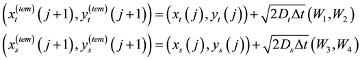 (2)
(2)
where ,
,  ,
,  , and
, and  are independent samples of standard normal distribution (mean 0, variance 1). To enforce the reflection condition at the boundary of the square search region, we calculate the new positions of target and searcher as
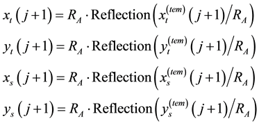 (3)
(3)
where function ![]() is defined as
is defined as
![]()
It is straightforward to verify that
![]() (4)
(4)
The target is labeled as “detected” at ![]() if the distance between the target and the searcher is less than the detection range R:
if the distance between the target and the searcher is less than the detection range R:
![]() (5)
(5)
Once the target is detected, that particular Monte Carlo run is terminated and another independent Monte Carlo run is started. To speed up the simulation, multiple Monte Carlo runs are carried out in parallel.
Let ![]() be the initial location of the searcher. In Monte Carlo simulations, the initial location of the target is selected randomly and uniformly from the part of the square search region that is outside the disk of radius R centered at
be the initial location of the searcher. In Monte Carlo simulations, the initial location of the target is selected randomly and uniformly from the part of the square search region that is outside the disk of radius R centered at ![]() (i.e., outside the the searcher’s detection area at
(i.e., outside the the searcher’s detection area at![]() ).
).
For each set of parameter values, we repeat the Monte Carlo run ![]() times. The non-detection pro- bability is calculated by averaging over 100,000 repeats.
times. The non-detection pro- bability is calculated by averaging over 100,000 repeats.
In Problem 1, we select the time step ![]() such that
such that
![]() (6)
(6)
That is, the root-mean-square of the displacement between the target and the searcher in time period ![]() is no more than one eighth of the detection radius of the searcher.
is no more than one eighth of the detection radius of the searcher.
We first examine the accuracy of our Monte Carlo simulations in the case of
![]()
Figure 2 compares the non-detection probabilities obtained with two different time steps: ![]() as given in (6) and
as given in (6) and![]() . Figure 2 demonstrates that the time step
. Figure 2 demonstrates that the time step ![]() is small enough. In Problem 1, we use
is small enough. In Problem 1, we use ![]() as the time step unless specified otherwise.
as the time step unless specified otherwise.
Figure 3 compares the non-detection probabilities obtained in 7 independent Monte Carlo simulations, each simulation consisting of ![]() repeats. The parameter set is the same as in Figure 2. From Figure 3, we can see that the number of repeats,
repeats. The parameter set is the same as in Figure 2. From Figure 3, we can see that the number of repeats, ![]() , is large enough.
, is large enough.
Next, we explore several cases that satisfy ![]() ranging from
ranging from ![]() to
to![]() . When
. When![]() , the searcher is fixed; when
, the searcher is fixed; when![]() , we have Dt = 0 and the target is fixed. The initial location of the searcher is
, we have Dt = 0 and the target is fixed. The initial location of the searcher is![]() .
.
Figure 4 plots the non-detection probability for various values of ![]() and
and![]() . The fastest decay of the non-detection probability occurs when
. The fastest decay of the non-detection probability occurs when ![]() (i.e., when the searcher is fixed at
(i.e., when the searcher is fixed at![]() ). The decay of
). The decay of
![]()
Figure 2. Comparison of numerical results obtained, respectively, with time step ![]() and refined time step
and refined time step![]() .
.
![]()
Figure 3. Comparison of results from 7 independent Monte Carlo simulations. Each simu- lation consists of ![]() repeats.
repeats.
![]()
Figure 4. Non-detection probability for various values of ![]() and
and![]() .
.
the non-detection probability is slowed down when the searcher diffuses with![]() . This observation indicates that the best location for the searcher is at the center
. This observation indicates that the best location for the searcher is at the center![]() ; diffusion with
; diffusion with ![]() randomizes the searcher location and decreases the decay rate of the non-detection probability. Notice that in Figure 4 when
randomizes the searcher location and decreases the decay rate of the non-detection probability. Notice that in Figure 4 when![]() , the decay rate of the non-detection probability is no longer sensitive to changes in
, the decay rate of the non-detection probability is no longer sensitive to changes in ![]() as along as
as along as ![]() is fixed. In other words, when both the searcher and target are diffusing, the decay rate of the non- detection probability is affected only by the relative diffusion
is fixed. In other words, when both the searcher and target are diffusing, the decay rate of the non- detection probability is affected only by the relative diffusion ![]() between the searcher and the target. Finally, in Figure 4, the slowest decay of the non-detection probability occurs when
between the searcher and the target. Finally, in Figure 4, the slowest decay of the non-detection probability occurs when![]() . Recall that the initial location of the target is randomized and is most likely away from the center.
. Recall that the initial location of the target is randomized and is most likely away from the center. ![]() fixes the target at its initial off-center location and makes it less likely for the diffusing searcher to encounter the target. In the case of
fixes the target at its initial off-center location and makes it less likely for the diffusing searcher to encounter the target. In the case of![]() , if we switch the roles of the target and the searcher, we see that when a searcher is fixed at an off-center location with no diffusion, the non-detection probability decays the slowest. Thus, for a given relative diffusion between the searcher and the target
, if we switch the roles of the target and the searcher, we see that when a searcher is fixed at an off-center location with no diffusion, the non-detection probability decays the slowest. Thus, for a given relative diffusion between the searcher and the target![]() , Figure 4 suggests the following observations:
, Figure 4 suggests the following observations:
1) the decay rate of the non-detection probability is the largest when the searcher is fixed at the center;
2) when both the searcher and the target are diffusing with significant diffusion coefficients, the decay rate of the non-detection probability is lower and is independent of ![]() as long as
as long as ![]() is a fixed constant;
is a fixed constant;
3) when the searcher is fixed at a location significantly off center, the decay rate of the non-detection probability is even lower.
To further test these observations, we compare the decay rates of the non-detection probability for 4 sets of parameters
![]()
Based on the observations 1)-3) above, we expect that set 1 produces the fastest decay of the non-detection probability; sets 2 and 3 yield similar decay rates, lower than that of set 1; and set 4 gives the slowest decay rate of the non-detection probabilty.
Figure 5 compares the results for these four parameter sets. The results in Figure 5 confirm what we predicted based on observations 1)-3). Hence, these results provide further support for observations 1)-3). Figure 5 also indicates that when the searcher has significant diffusion, its inital location does not matter.
Next we study the case of a fixed searcher![]() . We investigate how the searcher’s location affects the decay rate of the non-detection probability. Figure 6 shows that for a stationary searcher, the decay rate of the non-detection probability decreases as the distance between the searcher and the center is increased.
. We investigate how the searcher’s location affects the decay rate of the non-detection probability. Figure 6 shows that for a stationary searcher, the decay rate of the non-detection probability decreases as the distance between the searcher and the center is increased.
In summary, for Problem 1, we conclude that a) when both the searcher and the target have significant diffusion, the decay rate of non-detection probability is independent of the initial location and is independent of ![]() as long as
as long as ![]() is fixed; b) for a given value of
is fixed; b) for a given value of![]() , the fastest decay of non-detection probability occurs when the searcher is fixed at the center
, the fastest decay of non-detection probability occurs when the searcher is fixed at the center![]() .
.
Next, we study the case where the searcher moves with a constant velocity ![]() along a prescribed deterministic loop.
along a prescribed deterministic loop.
4. Problem 2: Searcher Moving along a Loop
We consider the situation where the target diffuses with diffusion coefficient ![]() and the searcher moves with velocity
and the searcher moves with velocity ![]() along a loop (a circular or a square loop). We select velocity
along a loop (a circular or a square loop). We select velocity ![]() as follows.
as follows.
Let ![]() be the time scale of the target diffusing a root-mean-square distance of 2R along a given direction. Time scale
be the time scale of the target diffusing a root-mean-square distance of 2R along a given direction. Time scale ![]() can be viewed as the time scale of the target probability distribution relaxing to erase the mark swept by the searcher. Time scale
can be viewed as the time scale of the target probability distribution relaxing to erase the mark swept by the searcher. Time scale ![]() is given by
is given by
![]() (7)
(7)
The distance traveled by the searcher with velocity ![]() in time period
in time period ![]() is
is![]() . We consider the regime
. We consider the regime
![]()
Figure 5. Comparison of decay rates of non-detection probability for 4 sets of parameter values.
![]()
Figure 6. The effect of the searcher location on the decay rate of non-detection probability when the searcher is fixed![]() .
.
where the target velocity is neither too small nor too large. Specifically, we consider the case where the distance traveled by the searcher in time ![]() is a small multiple of 2R:
is a small multiple of 2R:
![]() (8)
(8)
We pick![]() . The corresponding velocity is found to be
. The corresponding velocity is found to be
![]() (9)
(9)
In all the simulations below, we use![]() .
.
In Problem 2, for each set of parameter values, we repeat the Monte Carlo run ![]() times. We also use a smaller time step (see below). The increased time and ensemble resolution is made possible by the fact that when the searcher moves along a loop, the non-detection probability decays faster than in the optimal case of Problem 1 where the searcher is fixed at the center. With fast decay of the non-detection probability, detections occur early and consequently Monte Carlo runs on average end early in simulations.
times. We also use a smaller time step (see below). The increased time and ensemble resolution is made possible by the fact that when the searcher moves along a loop, the non-detection probability decays faster than in the optimal case of Problem 1 where the searcher is fixed at the center. With fast decay of the non-detection probability, detections occur early and consequently Monte Carlo runs on average end early in simulations.
We select the time step ![]() such that
such that
![]() (10)
(10)
That is, the root-mean-square diffusion of the target toward the searcher in time ![]() plus the distance traveled by the searcher in time
plus the distance traveled by the searcher in time ![]() does not exceed one twelfth of the detection radius of the searcher.
does not exceed one twelfth of the detection radius of the searcher.
We first examine the accuracy of our Monte Carlo simulations when the searcher moves along a circle of radius ![]() with velocity
with velocity![]() , as illustrated in the left panel of Figure 7.
, as illustrated in the left panel of Figure 7.
Figure 8 compares the non-detection probabilities obtained with two time steps: ![]() given in (10) and
given in (10) and![]() . Figure 8 tells us that the time step
. Figure 8 tells us that the time step ![]() is small enough. In Problem 2, we use
is small enough. In Problem 2, we use ![]() as the time step unless specified otherwise.
as the time step unless specified otherwise.
Figure 9 compares the non-detection probabilities obtained from 7 independent Monte Carlo simulations, each consisting of ![]() repeats. Figure 9 demonstrates that
repeats. Figure 9 demonstrates that ![]() is adequate for accurately capturing the decay of the non-detection probability.
is adequate for accurately capturing the decay of the non-detection probability.
Figure 10 shows the effect of the circle radius ![]() on the time evolutions of the non-detection probability. When the searcher moves along a small circle (small
on the time evolutions of the non-detection probability. When the searcher moves along a small circle (small![]() ), the non-detection probability decays moderately faster than in the case of the searcher being fixed at the center
), the non-detection probability decays moderately faster than in the case of the searcher being fixed at the center![]() . When we expand the circle path from
. When we expand the circle path from ![]() to
to![]() , to
, to ![]() the decay rate of the non-detection probability increases. The optimal radius for the fastest decay of the non-detection probability is about
the decay rate of the non-detection probability increases. The optimal radius for the fastest decay of the non-detection probability is about![]() . When the circle path is expanded beyond
. When the circle path is expanded beyond![]() , the decay rate of the non-detection probability is reduced slightly from the optimal value. When
, the decay rate of the non-detection probability is reduced slightly from the optimal value. When ![]() is large and the circle path is close to the boundary of the square search region, it takes long time for a target initially near the center to diffuse the long distance to encounter the searcher. Likewise, when
is large and the circle path is close to the boundary of the square search region, it takes long time for a target initially near the center to diffuse the long distance to encounter the searcher. Likewise, when
![]()
Figure 9. Comparison of results from 7 independent Monte Carlo simulations. Each simu- lation contains ![]() repeats.
repeats.
![]()
Figure 10. Results for the case of the searcher moving along a circle of radius![]() . Shown here are time evolutions of non-detection probability for various values of circle radius
. Shown here are time evolutions of non-detection probability for various values of circle radius![]() .
.
![]() is small and the circle path covers just the area near the center, it takes long time for a target initially near the boundary to diffuse the long distance to encounter the searcher. Thus, the optimal circle path is the one that is the best compromise for taking care both the area around the center and the area near the boundary of the search region. Intuitively, one may conjecture that the optimal circle path is the one that divides the whole search region into 2 equal parts:
is small and the circle path covers just the area near the center, it takes long time for a target initially near the boundary to diffuse the long distance to encounter the searcher. Thus, the optimal circle path is the one that is the best compromise for taking care both the area around the center and the area near the boundary of the search region. Intuitively, one may conjecture that the optimal circle path is the one that divides the whole search region into 2 equal parts:
![]()
The optimal circle radius based on the intuitive conjecture above is
![]() (11)
(11)
The results of Monte Carlo simulations in Figure 10 strongly support this conjecture.
Next we study the case of the searcher moving along a square path of half width ![]() with velocity
with velocity![]() , as illustrated in the right panel of Figure 7.
, as illustrated in the right panel of Figure 7.
Figure 11 shows the effect of half width ![]() on the time evolutions of the non-detection probability. When the searcher moves along a small square path (small
on the time evolutions of the non-detection probability. When the searcher moves along a small square path (small![]() ), the non-detection probability decays moderately faster than in the case of the searcher being fixed at the center
), the non-detection probability decays moderately faster than in the case of the searcher being fixed at the center![]() . When we expand the square path from
. When we expand the square path from ![]() to
to![]() , to
, to ![]() the decay rate of the non-detection probability increases. The optimal half width for fastest decay of the non-detection probability is about
the decay rate of the non-detection probability increases. The optimal half width for fastest decay of the non-detection probability is about![]() . When the square path is expanded beyond
. When the square path is expanded beyond![]() , the decay rate of the non-detection probability is reduced from the optimal value. When
, the decay rate of the non-detection probability is reduced from the optimal value. When ![]() is large and the square path is close to the boundary of the square search region, it takes long time for a target initially near the center to diffuse the long distance to encounter the searcher. Likewise, when
is large and the square path is close to the boundary of the square search region, it takes long time for a target initially near the center to diffuse the long distance to encounter the searcher. Likewise, when ![]() is small and the square path covers only the area near the center, it takes long time for a target initially near the boundary to diffuse the long distance to encounter the searcher. Intuitively, one may conjecture that the optimal square path is the one that divides the whole search region into two equal parts. Based on this intuitive conjecture, the optimal half width for the square path is given by
is small and the square path covers only the area near the center, it takes long time for a target initially near the boundary to diffuse the long distance to encounter the searcher. Intuitively, one may conjecture that the optimal square path is the one that divides the whole search region into two equal parts. Based on this intuitive conjecture, the optimal half width for the square path is given by
![]()
Figure 11. Results for the case of the searcher moving along a square of half width![]() . Shown here are time evolutions of non-detection probability for various values of half width
. Shown here are time evolutions of non-detection probability for various values of half width![]() .
.
![]() (12)
(12)
The results of Monte Carlo simulations in Figure 11 strongly support this conjecture.
Before we end this section, we calculate and compare the decay rates of the non-detection probability for the three optimal cases we have considered so far. The decay rate of the non-detection probability, denoted by![]() , is calculated by fitting a straight line to data points of time vs log(non-detction probability).
, is calculated by fitting a straight line to data points of time vs log(non-detction probability).
1) For the case of diffusing target and diffusing searcher with fixed total diffusion![]() , the optimal (the fastest) decay rate of the non-detection probability is achieved when the searcher is fixed at the center. The optimal decay rate is found to be
, the optimal (the fastest) decay rate of the non-detection probability is achieved when the searcher is fixed at the center. The optimal decay rate is found to be
![]()
2) For the case of the searcher moving along a circle of radius ![]() with velocity
with velocity![]() , the optimal (the fastest) decay rate of the non-detection probability is achieved when
, the optimal (the fastest) decay rate of the non-detection probability is achieved when![]() . The optimal decay rate is
. The optimal decay rate is
![]()
3) For the case of the searcher moving along a square of half width ![]() with velocity
with velocity![]() , the optimal (the fastest) decay rate of the non-detection probability is achieved when
, the optimal (the fastest) decay rate of the non-detection probability is achieved when![]() . The optimal decay rate is
. The optimal decay rate is
![]()
Out of these 3 cases, square loop of half width ![]() yields the fastest decay of the non-detection probability with decay rate
yields the fastest decay of the non-detection probability with decay rate![]() .
.
In the next section, we study the case where the searcher moves along a spiral.
5. Problem 3: Searcher Moving along a Spiral
We consider the situation where the target diffuses with diffusion coefficient ![]() and the searcher moves along a path consisting of rotated spiral loops, which we will describe in detail below. In all simulations of the searcher sweeping a prescribed path, we use velocity
and the searcher moves along a path consisting of rotated spiral loops, which we will describe in detail below. In all simulations of the searcher sweeping a prescribed path, we use velocity![]() . The selection of
. The selection of ![]() has been discussed in Problem 2. In Problem 3, we select numerical parameters as follows: each Monte Carlo simulation is repeated
has been discussed in Problem 2. In Problem 3, we select numerical parameters as follows: each Monte Carlo simulation is repeated ![]() times and the time step
times and the time step ![]() satisfies
satisfies
![]() (13)
(13)
The increase in number of repeats from ![]() to
to ![]() is made possible by that the detection is faster in Problem 3, and as a result, the Monte Carlo simulations, on average, end earlier than in Problems 1 and 2.
is made possible by that the detection is faster in Problem 3, and as a result, the Monte Carlo simulations, on average, end earlier than in Problems 1 and 2.
A spiral path is a sequence of rotated spiral loops and is specified by the number of revolutions ![]() in each spiral. The construction of a spiral path with
in each spiral. The construction of a spiral path with ![]() is shown in Figure 12. Each spiral loop in the spiral
is shown in Figure 12. Each spiral loop in the spiral
path is formed by a forward spiral starting at the origin and a backward spiral back to the origin. We use the Archimedean spiral. The forward spiral of ![]() revolutions can be mathematically described as
revolutions can be mathematically described as
![]()
We select the starting angle ![]() such that the ending angle
such that the ending angle ![]() is at a diagonal, pointing to a corner of the square search region (Figure 12(a)). For
is at a diagonal, pointing to a corner of the square search region (Figure 12(a)). For![]() , we select
, we select![]() ; for
; for![]() , we select
, we select![]() . The backward spiral is the mirror reflection image of the forward spiral with respect to the line of ending angle (Figure 12(b)). Mathematically the backward spiral is
. The backward spiral is the mirror reflection image of the forward spiral with respect to the line of ending angle (Figure 12(b)). Mathematically the backward spiral is
![]()
Recall that in our problem, the searcher moves along a path with a constant velocity. To use the spiral loop as the searcher’s sweeping path in simulations, we need to express ![]() as a function of arclength s. The arclength along the forward spiral is given by
as a function of arclength s. The arclength along the forward spiral is given by
![]() (14)
(14)
where function ![]() is the arclength in the special case of
is the arclength in the special case of ![]() and
and![]() :
:
![]() (15)
(15)
Let ![]() be the arclength of the forward spiral (half the arclength of the spiral loop). Mathematically, it follows that
be the arclength of the forward spiral (half the arclength of the spiral loop). Mathematically, it follows that
![]() (16)
(16)
For the forward spiral,![]() . The polar coordinates
. The polar coordinates ![]() of the forward spiral are expressed as functions of arclength s using the inverse function of
of the forward spiral are expressed as functions of arclength s using the inverse function of![]() .
.
![]() (17)
(17)
For the backward spiral,![]() . The polar coordinates
. The polar coordinates ![]() of the backward spiral are expressed as functions of arclength s as
of the backward spiral are expressed as functions of arclength s as
![]() (18)
(18)
In our numerical simulations, the inverse function ![]() is evaluated by solving for q in equation
is evaluated by solving for q in equation ![]() using Newton’s method.
using Newton’s method.
The Cartesian coordinates of the spiral loop as functions of arclength s are written out based on the polar coordinates:
![]() (19)
(19)
Next, we scale the spiral loop formed above to fit the square search region (Figure 12(c)). We scale the spiral loop by selecting the largest coefficient b that satisfies
![]() (20)
(20)
When sweeping the spiral loop, the Cartesian coordinates of the searcher as functions of time t are given by
![]() (21)
(21)
This is the formula we use to update the searcher location in simulations.
After finishing sweeping one spiral loop, the searcher rotates the spiral loop by ![]() and starts sweeping along the rotated spiral loop (Figure 12(d)). This process is repeated until the target is detected.
and starts sweeping along the rotated spiral loop (Figure 12(d)). This process is repeated until the target is detected.
Figure 13 demonstrates four spiral loops, respectively, of![]() , of
, of![]() , of
, of![]() , and of
, and of![]() . In each spiral loop, the forward spiral is shown in red and the backward spiral in blue. The corresponding spiral sweeping path for the searcher contains a sequence of rotations of the spiral loop.
. In each spiral loop, the forward spiral is shown in red and the backward spiral in blue. The corresponding spiral sweeping path for the searcher contains a sequence of rotations of the spiral loop.
Figure 14 depicts the time evolutions of the non-detection probability when the searcher sweeps various spiral paths. A spiral path is specified by![]() , the number of revolutions in the forward spiral. Figure 14 compares the results for 9 values of nrv, ranging from
, the number of revolutions in the forward spiral. Figure 14 compares the results for 9 values of nrv, ranging from ![]() to
to![]() . The fastest decay of the non-detection probability occurs at
. The fastest decay of the non-detection probability occurs at![]() . The decay rates are almost the same among
. The decay rates are almost the same among![]() ,
, ![]() , and
, and![]() . The spiral loop of
. The spiral loop of ![]() is shown in Figure 13(b). The corresponding spiral sweeping path is a sequence of ratations of the spiral loop. The decay rate of the non-detection probability at
is shown in Figure 13(b). The corresponding spiral sweeping path is a sequence of ratations of the spiral loop. The decay rate of the non-detection probability at ![]() is
is
![]()
We point out that the optimal decay rate given above for Problem 3 is faster (larger) than those of Problems 1 and 2.
6. Problem 4: Searcher Moving along a Square Spiral
Now we consider the situation where the target diffuses with diffusion coefficient ![]() and the searcher moves along a path consisting of rotated square spiral loops, which we will describe in detail below. The searcher moves with velocity
and the searcher moves along a path consisting of rotated square spiral loops, which we will describe in detail below. The searcher moves with velocity![]() , the same velocity as we used in Problems 2 and 3.
, the same velocity as we used in Problems 2 and 3.
In Problem 4, we use the same numerical parameters as in Problem 3: each Monte Carlo simulation is repeated ![]() times and the time step
times and the time step ![]() satisfies
satisfies
![]() (22)
(22)
A square spiral path is a sequence of rotated square spiral loops and is specified by the number of square layers ![]() in each forward square spiral. A square spiral loop is formed by a forward square spiral starting at the origin and a backward square spiral back to the origin.
in each forward square spiral. A square spiral loop is formed by a forward square spiral starting at the origin and a backward square spiral back to the origin.
We first focus on square spirals with unit inter-layer distance. A forward square spiral of ![]() square layers is
square layers is
![]()
Figure 14. Results for the case of searcher moving along various spiral paths. A spiral path is a sequence of ratations of a spiral loop and is specified by![]() , the number of revolutions in each forward spiral. Shown here are time evolutions of non-detection probability for various values of
, the number of revolutions in each forward spiral. Shown here are time evolutions of non-detection probability for various values of![]() .
.
described as follows. We cycle through 4 directions: positive x, positive y, negative x, negative y. If we start at ![]() and sequentially go in each of 4 directions by a distance of 1, we obtain a unit square with its lower left corner at
and sequentially go in each of 4 directions by a distance of 1, we obtain a unit square with its lower left corner at![]() . Mathematically, the construction of this unit square is concisely and conveniently denoted by
. Mathematically, the construction of this unit square is concisely and conveniently denoted by
![]()
With this simple notation, the forward square spiral of ![]() layers is described by
layers is described by
![]()
In this unit forard square spiral, the inter-layer distance is 1. Next we scale the unit forward square spiral to fit it to the search region. Let d be the inter-layer distance after the scaling. We select the inter-layer distance d as
![]()
where ![]() is the half width of the search region. All square spirals in Problem 4 are scaled using the inter-layer distance d given above. The forward square spiral of 2 layers
is the half width of the search region. All square spirals in Problem 4 are scaled using the inter-layer distance d given above. The forward square spiral of 2 layers ![]() is shown in Figure 15(a).
is shown in Figure 15(a).
We could select the backward square spiral as the mirror image of the forward square spiral with respect to
the line of angle![]() . If we do that, however, the backward square spiral will coincide with the forward square
. If we do that, however, the backward square spiral will coincide with the forward square
spiral in a substantial fraction of the path. Intuitively, that is not an efficient way of sweeping. We want the backward square spiral to cover the area between the layers of the forward square spiral so that together the forward and the backward square spirals have a better and more uniform coverage of the search region. We design the backward square spiral to go between the layers of the forward square spiral. Mathematically, the backward square spiral is described by
![]()
As in the situation for the forward square spiral, the backward square spiral is also scaled by the inter-layer distance d given above to fit it to the search region. The backward square spiral of 2 layers ![]() is shown in Figure 15(b) (blue line with filled circles). The square spiral loop is formed by combining the forward and the backward square spirals. The square spiral loop of
is shown in Figure 15(b) (blue line with filled circles). The square spiral loop is formed by combining the forward and the backward square spirals. The square spiral loop of ![]() is shown in Figure 15(b). The square spiral loop starts at the origin and returns to the origin at the end.
is shown in Figure 15(b). The square spiral loop starts at the origin and returns to the origin at the end.
After finishing sweeping the square spiral loop, the searcher rotates the whole square spiral loop by ![]() and starts sweeping along the rotated square spiral loop. This process is repeated until the target is detected.
and starts sweeping along the rotated square spiral loop. This process is repeated until the target is detected.
Figure 16 plots the time evolutions of the non-detection probability when the searcher sweeps various square spiral paths. A square spiral path is specified by![]() , the number of square layers in the forward square spiral (see Figure 15). Figure 16 compares the results for 9 values of
, the number of square layers in the forward square spiral (see Figure 15). Figure 16 compares the results for 9 values of![]() , ranging from
, ranging from ![]() (the lowest possible value for
(the lowest possible value for![]() ) to
) to![]() . The fastest decay of the non-detection probability occurs at
. The fastest decay of the non-detection probability occurs at![]() . The decay rates are almost the same among
. The decay rates are almost the same among![]() ,
, ![]() , and
, and![]() . The square spiral loop of
. The square spiral loop of ![]() is shown in Figure 15(d). The corresponding square spiral path is a sequence of ratations of the square spiral loop. The decay
is shown in Figure 15(d). The corresponding square spiral path is a sequence of ratations of the square spiral loop. The decay
![]()
Figure 16. Results for the case of the searcher moving along various square spiral paths. A square spiral path is a sequence of rotations of a square spiral loop and is specified by![]() , the number of square layers in each forward square spiral. Shown here are time evolutions of the non-detection probability for various values of
, the number of square layers in each forward square spiral. Shown here are time evolutions of the non-detection probability for various values of![]() .
.
rate of the non-detection probability at ![]() is
is
![]()
We point out that the optimal decay rate given above for Problem 4 is faster (larger) than those of Problems 1, 2 and 3.
7. Problem 5: Searcher Scanning Horizontally and Vertically
Finally we consider the situation where the target diffuses with diffusion coefficient![]() , and the searcher scans horizontally and vertically back and forth. The detailed construction of the scan path will be described below. The searcher moves with velocity
, and the searcher scans horizontally and vertically back and forth. The detailed construction of the scan path will be described below. The searcher moves with velocity![]() , the same velocity as we used in Problems 2, 3 and 4.
, the same velocity as we used in Problems 2, 3 and 4.
In Problem 5, we use the same numerical parameters as in Problems 3 and 4: each Monte Carlo simulation is repeated ![]() times and the time step
times and the time step ![]() satisfies
satisfies
![]() (23)
(23)
The scan path consists of forward horizontal scan, backward horizontal scan, forward vertical scan and backward vertical scan. A forward horizontal scan is shown in Figure 17.
A forward horizontal scan is specified by 3 parameters: b the length of each horizontal scan line, d the inter scan line distance, and ![]() the number of horizontal scan lines. Parameters b and d are shown in Figure 17. The distance from the first horizontal scan line to the last horizontal scan line is
the number of horizontal scan lines. Parameters b and d are shown in Figure 17. The distance from the first horizontal scan line to the last horizontal scan line is![]() . Since the searcher is scanning a square region, we set
. Since the searcher is scanning a square region, we set
![]()
For each forward horizontal scan, there is an associated backward horizontal scan. The backward scan travels between the horizontal scan lines of the forward scan. The forward horizontal scan is mathematically described by
![]()
The associated backward horizontal scan is mathematically described by
![]()
Figure 17. A forward horizontal scan and associated parameters. b is the length of each horizontal scan line; d is the vertical distance between adjacent scan lines.
![]()
![]()
![]()
The forward horizontal scan and the associated backward horizontal scan for ![]() are shown in Figure 18(a), Figure 18(b).
are shown in Figure 18(a), Figure 18(b).
The vertical scans are exactly the same as the horizontal scans except that the roles of x and y are swapped. The forward vertical scan is
![]()
The associated backward vertical scan is
![]()
Figure 18. Horizontal and vertical scan paths. (a) Forward horizontal scan; (b) Backward horizontal scan (blue line with filled circles); (c) Forward vertical scan; (d) Backward vertical scan (blue line with filled circles).
![]()
![]()
![]()
The forward vertical scan and the associated backward vertical scan for ![]() are shown in Figure 18(c), Figure 18(d).
are shown in Figure 18(c), Figure 18(d).
To scan the square search region of half width![]() , we set
, we set
![]()
Thus, for a square of given half width![]() , a scan path is completely specified by
, a scan path is completely specified by![]() , the number of scan lines in each scan.
, the number of scan lines in each scan.
The searcher sequentially cycles through forward horizontal scan, backward horizontal scan, forward vertical scan and backward vertical scan. This process is repeated until the target is detected.
Figure 19 shows the time evolutions of the non-detection probability when the searcher scans horizontally and vertically. A scan path is specified by![]() , the number of scan lines in each forward scan. Figure 19 compares the results for 9 values of
, the number of scan lines in each forward scan. Figure 19 compares the results for 9 values of![]() , ranging from
, ranging from ![]() (the lowest possible value for
(the lowest possible value for![]() ) to
) to![]() . The fastest decay of the non-detection probability occurs at
. The fastest decay of the non-detection probability occurs at![]() . The decay rates are almost the same among
. The decay rates are almost the same among![]() ,
, ![]() , and
, and![]() . The decay rate of the non-detection probability at
. The decay rate of the non-detection probability at ![]() is
is
![]()
Figure 19. Results for the case of searcher scanning horizontally and vertically. The horizontal and vertical scan paths are shown in Figure 18. A scan path is specified by![]() , the number of scan lines in each forward scan. Shown here are time evolutions of non-detection probability for various values of
, the number of scan lines in each forward scan. Shown here are time evolutions of non-detection probability for various values of![]() .
.
![]()
We point out that the optimal decay rate given above for Problem 5 is faster (larger) than those of Problems 1, 2, 3 and 4.
8. Summary
This paper calculated the non-detection probability of a diffusing target in the presence of a stationary or moving searcher. It is found that when the searcher is fixed, the decay rate of the non-detection probability attains the maximum value when the search is fixed at the center of the square search region. When both the searcher and the target diffuse with significant diffusion coefficients, the decay rate of the non-detection probability only depends on the sum of the diffusion coefficients of the target and searcher. When the searcher moves along various deterministic trajectories, the fastest decay of the non-detection probability is obtained when the searcher scans horizontally and vertically.
Acknowledgements and Disclaimer
Hong Zhou would like to thank Professor James Eagle, Professor Sivaguru Sritharan and Professor Jim Scrofani for stimulating discussions. The views expressed in this document are those of the authors and do not reflect the official policy or position of the Department of Defense or the US Government.