Analysis on a Mathematical Model for Tumor Induced Angiogenesis ()
1. Introduction
Tumor Angiogenesis is the process by which cancerous cells signal surrounding blood capillaries to initiate the formation of new red blood cells. These new capillaries gradually form a dendritic structure and spread through the extra cellular matrix. The red blood vessels grow progressively over time towards the local tumor mass under the influence of chemical stimuli such as vascular endothelial fibroblast growth factors (VEGF) or basic fibroblast growth factors (BFGF) [1] -[4] . The chemical agents that contribute to the process of angiogenesis come from a source, located usually in the necrotic, proliferating or both regions of the local tumor [5] [6] . It is a well established fact that unvascularized tumors cannot grow beyond 2 mm and are not likely to metastasize. This has been proved experimentally by Judah Folkman et al. [7] . Since the publication by Judah Folkaman several hypothesis and research have been conducted to investigate the possibility of controlling angiogenesis in the case of cancerous cells. Our research can play a role in understanding the challenge that angiogenesis presents by studying the influence of the source of growth factors in angiogenesis.
By introducing a source term into the PDE model, we extend the model proposed by H. A. Harrington et al. [8] . The model describes how tumor angiogenic factors from a source influences the growth of red blood cells in the direction of the tumor. It also assesses the interplay between tumor angiogenic inhibitor and the tumor angiogenic factors.
We assume that the source term depends on time and a location in the tumor (most likely the necrotic region, proliferating cells or both) which induces tumor angiogenic growth factors (TAF), such as vascular endothelial growth factors (VEGF) or basic fibroblast growth factors (BFGF). The proposed source term  is a function of the form;

 represents the time it takes the tumor to initiate new signaling growth factors. For
  large enough, our model reduces to H. A. Harrington’s model. The threshold needed to signal growth factors from the source term,
  is assumed to be a constant value for simplicity and lack of experimental data. Figure 1 is a cartoon diagram of the model as described in the previous paragraphs.
In order to mimic the experimental work by Folkman et al., we adapted Figure 2 as observed in [8] [9] . Our model as mentioned earlier is a modified form of Harrington’s model. We proposed a similar model by adding a source term which depends on a threshold parameter, time. We described the diffusion and inhibition of tumor angiogenic factors using partial differential equations on a two dimensional plane. In Figure 3, the diamond region represents the source of the tumor angiogenic factors whose initiation depends on the threshold parameter, time.
We shall take a look at a hybrid model for tumor induced angiogenesis at the tissue level. As described previously, our model describes the diffusion of tumor angiogenic factors within the extra cellular matrix and how red blood vessels respond to these factors by growing towards the tumor along the gradient of the chemical stimuli.
The contents of the paper are divides as follows; section 2 describes the general form of the model and its parameters. In section 3 we discuss the numerical methods used in solving the system. In section 4 we compute numerically the PDEs arising from the model and conclude in section 5 with a summary of our results and some future directions.
2. Model Description
We assume that the process of angiogenesis is spatially homogeneous, thus we can model the spread and interaction of the coupled tumor angiogenic and inhibitor factors within the extracellular matrix with a source term using ordinary differential equations. Although the ordinary differential equation model does not capture all the details of angiogenesis, it is a good starting point to understand its dynamics. The ordinary differential equation model is as follows;
 (1)
(1)
 (2)
(2)
with initial conditions;
 (3)
(3)
 (4)
(4)
where  and
and  are state variables representing the concentrations of tumor angiogenic factor (TAF) and inhibitor respectively, and
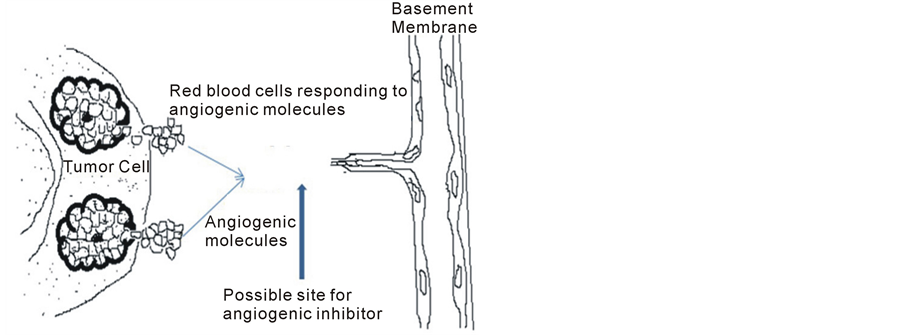
Figure 1. Diffusion of tumor angiogeneic factors and response of endothelial cells in the direction of the tumor angiogenic factors. The vertical arrow shows a possible location where an inhibitor can be introduced. The Tumor cells on the right hand side represent the source from which the signaling factors are induce from. The signaling factors are induced at some given time intervals.
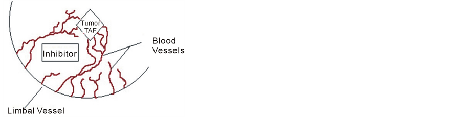
Figure 2. The following diagram mimics the interaction between tumor induced angiogenic factors and an inhibitor in the cornea. Proliferating blood vessels from the limbal vessel are avoid the path where the inhibitor has been introduced. Blood vessels growing towards tumor in response to tumor angiogeneic factors.

Figure 3. The above diagram is an 8 × 8 square which represents the region where the interaction between tumor angiogenic factors and inhibitors occur. The shaded rectangle in the square, represents the initial concentration of tumor angiogenic factors and location of source term. The diamond region represents the initial concentration of inhibitor.

represents a source term which depends on time.  and
and  represent initial concentration of tumor angiogenic factor and inhibitor respectively. The parameters in the ordinary differential equations (1) and (2) are constants obtained from previous literature [8] [9] are described in detail in Table1 The function
  is obtained

Table 1 . Parameter values for the PDE and ODE model. These values were Taken from previous literature [4] and [5] .
artificially due to the lack of experimental data. The following graphs displays our results from solving equations (1)-(4).
Ordinary differential equation models as mentioned earlier are not enough to capture the dynamics of spatially heterogeneous biological behavior. We therefore include a spatial term and study the dynamic of the system within this frame work. The partial differential equations are modeled from the results of Harrington et al. by adding a source term to their equations. We impose Dirichlet boundary and initial conditions on the system as follows;
 (5)
(5)
 (6)
(6)
where the parameters  and
and  represents the diffusion rate constant for TAFs and inhibitors respectively. Similarly the parameter
  is the natural inactivation rate of the TAF’s while the parameters
  and
and  is the capillary indicator function which depends on time and the location where the tumor is source is located. Lastly the parameter
  is the rate constant controlling the relationship between the TAF’s and the inhibitors.
3. Discussion of Numeical Method—Explicit Stabilized Runge-Kutta Methods
Some recent and older publications in [10] -[13] showed that explicit stablized Runge Kutta methods possess extended stability domains and have less restriction on the choice of their step size as compared to the more classical Runge-Kutta methods. This property thus makes explicit stabilized runge kutta methods good options to consider when solving partial differential equations numerically, much as implicit methods are the more desirable choice. It has been shown by Assyr Abdulle [10] that the explicit stabilized Runge-Kutta schemes work very well for mildly stiff system. The model under consideration is mildly stiff and thus it is reasonable to use explicit stabilized methods.
An extensive discussion on the construction and how to implement the methods can be found in [10] -[14] . We however provide here a more concise overview to motivate the implementation of this method to our model. This discussion is not a substitute to reading on the more elaborate technical report by Assyr Abdulle on the subject and other text book material. The general idea for the construction of the methods can be divided into two steps:
Construct Stability polynomials bounded in a long strip around the negative real axis.
Develop a numerical methods which has such favorable stability functions.
The first step to achieving the steps mentioned above will be to generate an optimal stability polynomial of order  and degrees
  of the form

such that  and
and .
.
It has been shown by [14] that polynomials of this type for arbitrary  and
and  values exists and are unique. Riha’s approach to constructing such polynomials is very analytical in nature and is not used very much in practice. A more friendly approach to constructing these polynomials is the use of numerical approximations. Some numerical approximations which have been used to construct some of these polynomials include DUMKA method, Runge-Kutta Cheybyshev method and the optimal Runge-Kutta Chebyshev method (ROCK). These methods are what we seek to employ in solving our system and consequently test how well they perform as they have not been widely used as compared to the more traditional implicit methods. We will discuss in the next subsections the DUMKA method and the optimal Runge-Kutta Chebyshev method. We use these methods in solving our model numerically.
3.1. Dumka Method
DUMKA method is computed through an iterative procedure which is based on the zeros of the optimal stability polynomials. Optimal stability polynomials can be thought of as the generalized Chebyshev polynomials. There are a lot of literature discussion on this subject a very good source can be found in [15] . Every step leading to the solution under this method consists of a two stage scheme. This approach helps reduce error propagation that can arise when solving differential equations numerically. One general approach for solving time-dependent partial differential equations is to discretize the space variables to obtain a system of ordinary differential equations of the form , where,
 and
and  has a value in
 . The general form of the DUMKA method for solving the resulting system of ordinary differential equation is given as follows;


where  is an initial condition,
  is the time step,
  are the zero’s of the optimal stability polynomials and
  are the squares of the zero’s of the optimal stability polynomials.
  is called the internal stages and are constructed by composition. This can be composition of
  explicit Euler methods. The interested reader should refer to [14] -[16] for more in depth discussion on the method.
3.2. Rock Method
The ROCK method is built on a recurrence relation and has been derived for orders  and
and . In [16] , the author proved that the optimal stability polynomials of even orders have exactly
  complex zeros. In the construction of the ROCK method, the first thing we do is to look for some
  from the family of polynomials, such that the approximation to the optimal stability polynomial is given as;
 (7)
(7)
 (8)
(8)
where  is a member of a family of polynomials
 , which are orthogonal to the weight function
 and the zeros of
  are closely or approximately equal to the
  complex zeros of equation (2).
The theoretical frame work of equation (1) is based on Bernstein’s Theorem.
Due to the recurrence relation of orthogonal polynomials , a method based on recurrence formula can be constructed.
Next we shall look at the construction of the approximate polynomial to Equation (1) for  such that

The three-term recurrence formula associated with the polynomials  where
where

can be used to determine the internal stages of the ROCK method defined as
 (9)
(9)
 (10)
(10)
and

The final structure of the method is as follows


In a similar fashion of derivation, the fourth order ROCK method is given as follows


In this paper we apply the schemes discussed above that is the DUMKA method and the second and fourth order optimal Runge-Kutta Chebyshev method (ROCK-2, ROCK-4) on the hybrid model for tumor induced angiogenesis. As mentioned earlier the above discussion is not a substitution for reading the references [14] -[16] and additional books. The reader who is interested in explicit stabilized numerical methods should read further on the subject as noted.
4. Results and Discussion
We now take a look at the results obtained from the application of the explicit stabilized Runge-Kutta methods on the 2-dimensional partial differential equation model for tumor angiogenesis. The model together with its initial and Dirichlet boundary conditions as mentioned earlier are given as follows;
 (11)
(11)
 (12)
(12)
with initial conditions


We note that the parameter values 4.0, 2.5, 0.4, 1.0, 10.0 and 5.5 together with the domain are arbitrarily chosen. We would have liked, to have chosen these values from experimental data but none was immediately available to us.
The following graphs are solutions of the system of partial differential equations (11) and (12) together with the initial conditions. These solutions represent the diffusion of the tumor angiogenic factors and the tumor angiogenic factor inhibitors within the extra cellular matrix. We realized that the behavior of the system closely matches what the literature suggests. That is in the presence of the inhibitors, the concentration of the tumor angiogenic factors is suppressed whiles the inhibitors remain within the system under consideration.
We also looked at the case where the inhibitor is placed at a different position by changing the initial condition slightly and check its effect on the tumor angiogenic factors. The location of the inhibitor relative to the tumor angiogenic factors is important. This is because it appears the inhibitor has to be located close enough to the tumor source in order to have an effect on the tumor angiogenic factors.
Lastly, we considered the effect of a source term ; which is a function of time and a threshold value. As mentioned earlier the threshold value determines the effect that the source term has on the model under consideration. The plots below represent the L1 and L2 norms respectively of the solutions of the system (11)-(12) with respect to varying threshold values.
Finally the computational times of the three explicit stabilized Runge-Kutta methods is reported in table 2.
From the results reported in Table 2 from the numerical computation, the ROCK2 out performs the ROCK 4 method in terms of computational speed and number of functional evaluations. This is consistent with the theory since ROCK2 has less stages than the ROCK4 method as mentioned previously in the discussion section.
5. Conclusions and Future Work
We extended the model of Harringtionby adding a time dependent source term of the form
The source term models the signaling of growth factors from the tumor, to recruit red blood vessels: which depends on a threshold parameter,  (represents the time it takes the tumor to initiate signaling growth factors) to facilitate the process of angiogenesis.
We believe our results will provide some answers to some questions arising from angiogenesis. For example, experimentalist can use the threshold parameter,  to characterized aggressive tumors and non-aggressive tumors. This is because our results indicate that if
  is large enough, there is a long delay of initiating the growth factors. Thus we categorize these tumors to be non-aggressive. On the other hand, if
  is small, angiogenesis is initiated quickly and we categorize this as aggressive tumors (For example in Figures 4-8, small threshold implies high tumor angiogenic factors).
We used three explicit stabilized Runge-Kutta methods for solving the extended mathematical model for tumor induced angiogenesis in the cornea.
In our model we used a simple geometry as shown in Figure 3. We will like to explore into more complex geometries. In the future, we will like to use Splines instead of methods of lines (which is used for the discreteTable2 Computational times for the different numerical methods for varying time steps tau is reported below.
Table 2. Computational times for the different numerical methods for varying time steps tau is reported below.

Figure 4. Represents the solution profile for the ode model at 4 different threshold values. The threshold values  are 0.05, 0.3, 0.55 and 0.8 respectively. The dashed lines represents the solution profile of the inhibitor and the solid line represents the profile of the tumor angiogenic factors.

Figure 5. Concentration Profiles of tumor angiogenic factors (TAF) and Inhibitor. The following profile is a snap shot of the diffusion of TAF and inhibitor concentration at the end of the time interval.
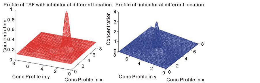
Figure 6. The following profile is a snap shot of the diffusion of TAF and inhibitor concentration. In this model, the initial position (initial condition) of the tumor angiogenic factors and the inihibitor profile was changed.

Figure 7. L1 norm Vs varying threshold values. This plot show that for a small threshold value, there is a high concentration of the tumor angioegenic factors.
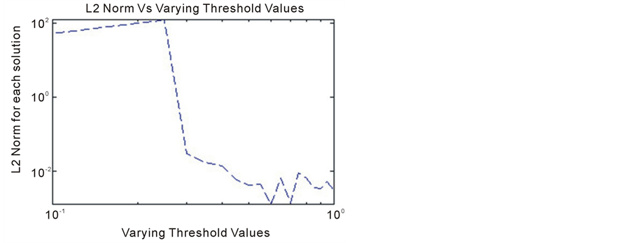
Figure 8. L2 norm Vs varying threshold values. The plots of the L2-norm suggests a similar phenomenon. That is the threshold parameter has a strong influence on the behavior of the solution.
zation in the explicit stabilized Runge-Kutta Methods) to reduce the system partial differential equations to ordinary differential equations. The use of Splines will lower the number of odes to be solved and consequently the system can be solved much faster. We are currently working on obtaining experimental data to perform a parameter estimation on the model. It is our hope that we can extend the current tissue scale model (PDE) to include both cellular (ODE) and sub-cellular dynamics (individual based model). In the extension we will like to consider as well, functional coefficients for the diffusion parameter.