High Order Central Schemes Applied to Relativistic Multi-Component Flow Models ()
1. Introduction
In recent years, relativistic gas dynamics plays an important role in areas of astrophysics, high energy particle beams, high energy nuclear collisions, and free-electron laser technology. The equations that describe the relativistic gas dynamics are highly nonlinear. For the practical problems, it is difficult to solve these equations analytically, therefore numerical solutions are perused. Several numerical methods for solving relativistic gas dynamics have been reported. All these methods are mostly developed out of the existing reliable methods for solving the Euler equations of non-relativistic or Newtonian gas dynamics.
The first attempt to solve the equations of relativistic gas dynamics (RGD) was made by Wilson [1] [2] using an Eulerian explicit finite difference code with monotonic transport. The code relies on artificial viscosity technique [3] to handle shock wave. Despite of its popularity it turned out to be unable to accurately describe the extremely relativistic flows [4] . In mid eighties, Norman and Winkler [5] proposed a reformulation of the difference equations with artificial viscosity consistent with relativistic dynamics of non-perfect fluids. Dean et al. [6] used flux correcting algorithms for RGD equations in the context of heavy ion collisions.
A good introduction about the recent methods applied to RGD can be found in the review article of Martí and Müller [7] . Some popular methods which are extended for RGD and are also discussed in [7] are the Rao methods [8] used by Eulderink et al. [9] [10] , PPM method [11] by Martí and Müller [12] , Glimm’s methods [13] by Wen et al. [14] , HLL method [15] by Schneider et al. [16] , Marquina flux formula [17] by Martí et al. [12] [18] and relativistic beam scheme [19] by Yang et al. [20] .
The development of numerical methods for the non-relativistic multi-component flows have attracted much attention in the past years, for example Fedkiw et al. [21] [22] , Karni [23] -[25] , Karni and Quirk [26] , Marquina and Mulet [27] . Moreover, Xu [28] used BGK-based gas-kinetic schemes to solve multi-component flows, while Lian and Xu [29] used the same scheme in order to solve the multi-component flows with chemical reactions.
This paper is an extension of the relativistic Euler equations to multi-component flows. We use the high-resolution non-oscillatory central schemes of Nessyahu and Tadmor [30] as well as Jiang and Tadmor [31] to solve these Euler equations. In this study, we consider only two-component flow, however, an extension to further components will result in addition of a continuity equation for the corresponding species. The central schemes are predictor-corrector methods which consist of two steps: starting with given cell averages, we first predict point values which are based on the non-oscillatory piecewise-linear reconstructions from the cell averages. At the second corrector step, we use staggered averaging, together with the predicted mid values, to realize the evolution of these averages. This results in a second-order, non-oscillatory central scheme.
The second order accuracy of these schemes is based on MUSCL-type reconstruction. Like upwind schemes, the reconstructed piecewise-polynomials used by the central schemes, also make use of non-linear limiters which guarantee the overall non-oscillatory nature of the approximate solution. But unlike the upwind schemes, central schemes do not require the intricate and time-consuming (approximate) Riemann solvers which are essential for the high-resolution upwind schemes. This advantage is especially important in the multi-dimensional case where there is no exact Riemann solver. Moreover, the central schemes are “genuinely multi-dimensional” in the sense that it does not necessitate dimensional splitting. Apart from these, central schemes do not produce spurious oscillations, such as carbuncle phenomena and odd-even decoupling which usually happens in the Godunov upwind schemes. The reason of this advantage is the presence of sufficient numerical dissipation in the central schemes. This is also the reason here in the multi-component flow that we see almost negligible or no oscillations at the gases interface [32] .
The organization of this paper is as follows. In Section 2, we derive the three-dimensional Euler equations for the relativistic multi-component flows. We then discuss how to obtain the primitive variables from the conserved variables. In Section 3, we write the one-dimensional relativistic Euler equations for the dynamics of a mixture of two gases. Starting from the first order central scheme, we explain the high-resolution second order central schemes to solve these Euler equations, see [30] and references therein. In Section 4, we explain the scheme for the two-dimensional relativistic multi-component flows. We again start from the first order central schemes and then extend it to second order, see [31] and references therein. In Section 5, we present numerical test cases which include propagation of one-dimensional (1D) relativistic blast waves, collision, cylindrical explosion, interaction of an air shock with helium bubble and explosion in a square box. Finally, Conclusion is given in Section 6.
2. Multi-Component Relativistic Euler Equations
For simplicity, we assume a model of mixture of two gases. An extension to more components is analogous. Let  denotes the total density of a mixture, with
  and
and  as the rest mass densities of the first and second components, respectively. Also let
  and
and  be the mass fractions of the first and second components. We assume that both components are in thermal equilibrium and are perfect gases with specific heats at constant volume
 ,
,  , specific heats at constant pressure
 ,
,  and ratios of specific heats
 ,
, . By standard thermodynamic arguments, the ratio of specific heats
  of the mixture of gases is
 (1)
(1)
Using the Einstein summation convention the equations describing the motion of a two-component relativistic fluid are given by the six conservation laws
 (2)
(2)
where  and
and  denote the covariant derivative with respect to coordinate
 . Furthermore,
  is the four-velocity of the mixture, and
  is the stress-energy tensor, which for a perfect fluid can be written as
 (3)
(3)
Here  is metric tensor

 is the mixture density, p the fluid average pressure, and h the specific enthalpy of the fluid mixture defined by
 (4)
(4)
where  is the specific internal energy. Note that we use natural units (i.e., the speed of light
 ) throughout this study. In Minskowski space time and Cartesian coordinates
 , the conservation equations given in Equation (2) can be written as
 (5)
(5)
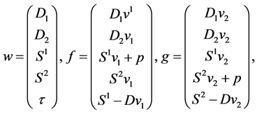
with the conserved variables w and fluxes  given as
 (6)
(6)
The six conserved quantities  and
and  are the rest-mass densities of the two components, the three components of momentum density, and the energy density (measured relative to the rest mass density), respectively. They are all measured in laboratory frame, and are related to quantities in the local rest frame of the fluid (primitive variables) through the relations
 (7)
(7)
where  are the components of three-velocity of fluid

with the Lorentz factor . Let us define
  as
as
 (8)
(8)
Note that , because
  The system of equations in Equation (5) along with definitions in Equations (6)-(8) is closed by mean of an ideal equation of state (EOS) as given below
 (9)
(9)
We denote by  the sound speed, defined by
 (10)
(10)
where s is the specific entropy, which is conserved along fluid lines. For EOS under consideration the speed of sound can be written as
 (11)
(11)
The Mach number of the flow is due to Königl [33]

For any given initial macroscopic variables in space and time,
 (12)
(12)
The common values of density , velocity
 , and pressure p can be obtained from the conservation requirements,
 (13)
(13)
From the above equations p,  and
and  can be obtained by first solving an implicit function of pressure whose zero represents the pressure [7] [34] . We have to find the root of the equation
 (14)
(14)
with
 (15)
(15)
The monotonicity of  ensures the uniqueness of the solution. The lower bound of the physically allowed domain,
  , defined by
 (16)
(16)
is obtained from Equation (7) by taking in to account that (in our units) . Knowing p, Equation (15) then directly gives v and density. Similar to Aloy et al. [34] , we obtained the solution
  by means of Newton-Rahphson iteration in which the derivative of
 , i.e.
 , is approximated by
 (17)
(17)
where  is the speed of sound given by
 (18)
(18)
This approximation tends to the exact derivative when the solution is approached. On the other hand, it easily allows one to extend the present algorithm to general equation of state [34] .
3. One-Dimensional Multi-Component Flows
Here, we are looking for spatially one-dimensional solutions of the two-component relativistic Euler equations. We only consider the solutions which depend on t and  and satisfy
 ,
,  ,
,  ,
,  and
and . The three dimensional system in Equation (2) then reduces to
 (19)
(19)
with the conserved variables w and fluxes f given as
 (20)
(20)
where
 (21)
(21)
and
 (22)
(22)
where . For any given initial macroscopic variables in space and time,
 (23)
(23)
the common values of density , velocity v, and pressure p can be obtained from the conservation requirements,
 (24)
(24)
From the above equations p,  , and v can be obtained by following the same procedure as given in relations (8)-(11).
3.1. One-Dimensional Central Schemes
Let us begin by introducing the well-known first order Lax-Friedrichs (LxF) scheme for one-dimensional conservation laws. This first order scheme is then extended to a second order central scheme, see [30] . We consider a piecewise-constant initial data,  , where,
  is a characteristic function of the cell,
 , centered around
 . Integrating Equation (19) over the rectangle
 , we get

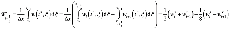
Note that our cells  are staggered with respect to the interval
  of integration. This leads to the LxF scheme
 (25)
(25)
where . The piecewise constant cells in each step are staggered with respect to those in the previous step.
3.2. Extension to Higher Order
Starting with a piecewise-constant solution in time and space,  , one reconstruct a piecewise linear (MUSCL-type) approximation in space, namely
 (26)
(26)
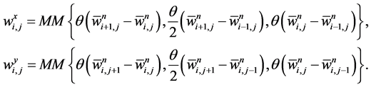
where  abbreviates a first-order discrete slopes, see Figure 1. A possible computation of these slopes, which results in an overall non-oscillatory scheme (consult [30] ), is given by family of discrete derivatives parameterized wit
 , i.e., for any grid function
  we set
 (27)
(27)
Here,  denotes the central differencing,
  , and MM denotes the min-mod nonlinear limiter
 (28)
(28)
This interpolate, is then evolved exactly in time and projected on the staggered cell-averages on the next time step, .
.
Consider the balance law over the control volume , we have

This yields
 (29)
(29)
Here, . The averaging of the linear data in Equation (26) at
 , yields
 (30)
(30)
So far everything is exact. Moreover, the Courant-Friedrichs-Levy (CFL) condition guarantees that  and
and , are smooth functions of
 ; hence they can be integrated approximately by the midpoint rule at the expense of an
  local truncation error. Thus we can write
 (31)
(31)
Putting Equation (31) in Equation (30), we finally get
 (32)
(32)
By Taylor expansion and the conservation laws in Equation (19), we have
 (33)
(33)
This may serve as our approximate mid-values  within the permissible second-order accuracy requirement. Here,
  stands for an approximate numerical derivatives of the flux
 ,
,
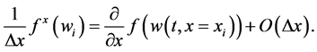
The fluxes  are computed by applying the min-mod limiter to each of the component of f, i.e.,

Here,  denotes the central differencing,
 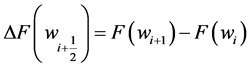 , and MM denotes the min-mod nonlinear limiter given by Equation (28). This component wise approach is one of the main advantages offered by central schemes over corresponding characteristic decompositions required by upwind schemes [30] [31] . It is important to emphasize that while using the central type LxF solver, we integrate over the entire Riemann fan, which consists of both the left and right going waves. On the one hand, this enables us to ignore the detailed knowledge about the exact (or approximate) generalized Riemann solver. On the other hand, this enables us to accurately compute the numerical flux, whose values are extracted from the smooth interface of two non-interacting Riemann problems.
In summary, this family of central differencing scheme takes the easily implemented predictor-corrector form,
 (34)
(34)
 (35)
(35)
4. Two-Dimensional Multi-Component Flows
Here we are looking for spatially two-dimensional solutions of the multi-component Euler equations. We only consider the solutions which depend on t,  ,
,  and satisfy
 ,
,  ,
,  ,
,  and
and . The three-dimensional system in Equation (5) then reduces to
 (36)
(36)
The conserved variables w and fluxes f, g are given by
 (37)
(37)
where
 (38)
(38)
and
 (39)
(39)
Here, . For any given initial macroscopic variables in space and time,
 (40)
(40)
The common values of density , velocity
 , and pressure p can be obtained from the conservation requirements,
 (41)
(41)
From the above equations p,  and
and  can be obtained by following the same procedure as given in Equations (7)-(11).
4.1. Two-Dimensional Central Schemes
To approximate Equation (36), we begin with a piecewise constant solution . We denote by
 , the approximate cell-average at
 , associated with the cell
 , centered around
 , i.e.
 (42)
(42)
and  is a characteristic function of the cell
 .
.
The arguments applied to the one-dimensional case can be easily extended to the higher dimensions. In the following, we will abbreviate to denote the normalized integral, i.e., normalized over its length, area, etc. Also let
 and
and  denote the fixed mesh-ratio in the xand y-directions, respectively. Let

denote the staggered averages. Integrating Equation (36) over the volume , we get [31]
 (43)
(43)
As given in Figure 2, the first integral has contribution from the four cells ,
, 
 , and
, and . Simplifying the above balance law we finally get the following LxF scheme [31]
 (44)
(44)
4.2. A Second-Order Extension in 2D
A two-dimensional extension of the second order central scheme was introduced in [31] . As in one-dimensional case, this staggered scheme can be viewed as an extension to the first-order LxF Scheme. A piecewise-linear interpolant is reconstructed from the calculated cell-averages at time ,
,
 (45)
(45)
Here  and
and  are discrete slopes in the xand y-directions, respectively, which are reconstructed from the given cell averages. To guarantee second-order accuracy, these slopes should approximate the corresponding derivatives,
 (46)
(46)
A possible computation of these slopes, which results in an overall non-oscillatory schemes is given by family of discrete derivatives parameterized with , for example

Figure 2. Floor plane of the staggered grid.
 (47)
(47)
Here MM denotes the min-mod nonlinear limiter given by Equation (28). This guarantees that the corresponding piecewise-linear reconstruction in Equation (45),  , is co-monotone with the underlying piecewise-constant approximation,
 . Similar to one-dimensional case, the construction of the central scheme proceeds with a second step of an exact evolution. The integration of Equation (36) over volume
  yields [31]
 (48)
(48)
We begin by evaluating the cell average . It has contribution from the four intersecting cells,
  ,
, 
 and
and  Starting with the intersecting cell
  at the corner (see Figure 2),
  , we find an average of the reconstructed polynomial in (45),
 (49)
(49)
Continuing in a counter clockwise direction, we have
 (50)
(50)
 (51)
(51)
 (52)
(52)
By adding the last four integrals, we find that the exact staggered averages of the reconstructed solution at .
.
 (53)
(53)
So far everything is exact. We now turn to approximating the four fluxes on the right of Equation (48), starting with the one along the east face (consult Figure 3), i.e.

We use midpoint quadrature rule for second-order approximation of the temporal integral,
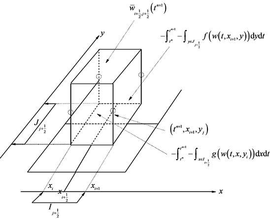
Figure 3. The central, staggered stencil.

and, for the reasons to be clarified below, we use the second-order rectangular quadrature rule for the spatial integration across the y-axis, yielding
 (54)
(54)
In similar manner, we approximate the remaining fluxes,
 (55)
(55)
 (56)
(56)
 (57)
(57)
The fluxes in Equations (54)-(57) use the midpoint values,  , and we take advantage of utilizing these mid-values for the spatial integration by the rectangular rule. Namely, since these mid-values are secured at the smooth center of their cells,
  , bounded away from the jump discontinuities along the edges, we may use Taylor expansion,

Finally, we use the differential form of conservation laws in Equation (36) to express the time derivative,  , in term of the spatial derivatives,
  and
and ,
,
 (58)
(58)
Here,

are one-dimensional discrete slopes of the fluxes in the xand y-directions, of the type reconstructed in Equation (46). We find these slopes in the same way as done for the conservative filed variables using min-mod procedure. Inserting these values, together with the staggered averages computed in Equation (53), into Equation (48), we get new staggered averages at 
 (59)
(59)
In summary, we end up with a simple two-step predictor-corrector scheme in Equations (58) and (59). Starting with the cell averages,  , we use the first-order predictor in Equation (58) for the evolution of the midpoint values,
  , which is followed by the second-order corrector in Equation (59) for computation of the new cell averages,
  This results in a second-order accurate non-oscillatory central schemes. As in the onedimensional case, no exact (approximate) Riemann solvers are involved. The non-oscillatory behavior of the scheme things on the reconstructed discrete slopes,
  ,
,  ,
,  and
and 
5. Numerical Test Cases
Here we present oneand two-dimensional numerical problems in order to validate the application of central schemes for the solution of multi-component flow problems.
Problem 1: Propagation of relativistic blast waves:

where the computational domain  is subdivided into 400 mesh points. This test problem has been considered by several authors in one-component case, for example, Hawley, Smarr and Wilson [35] , Schneider et al. [16] , and Martí and Müller [7] [12] , etc. It involves the formation of an intermediate state bounded by a shock wave propagating to the right and transonic rarefaction wave propagating to the left. The fluid in the intermediate state moves at a mildly relativistic speed (
 ) to the right. Flow particles accumulate in a dense shell behind the shock wave compressing the fluid by a factor of 5 and heating it up to values of internal energy much larger than the rest-mass energy. Hence the fluid is extremely relativistic in thermo-dynamical point of view, but mildly relativistic dynamically. The results are shown in Figure 4.
Problem 2: The initial data are:

where the computational domain is  with 400 mesh points. This problem was first considered in single-component case by Norman and Winkle [36] . The flow pattern is similar to that of problem 1, but more extreme as shown Figure 5. In case of 4000 mesh points the relativistic effects reduces the post-shock state to a thin dense shell with a width of only about 2% of the grid length at t = 0.35. The fluid in the shell moves with
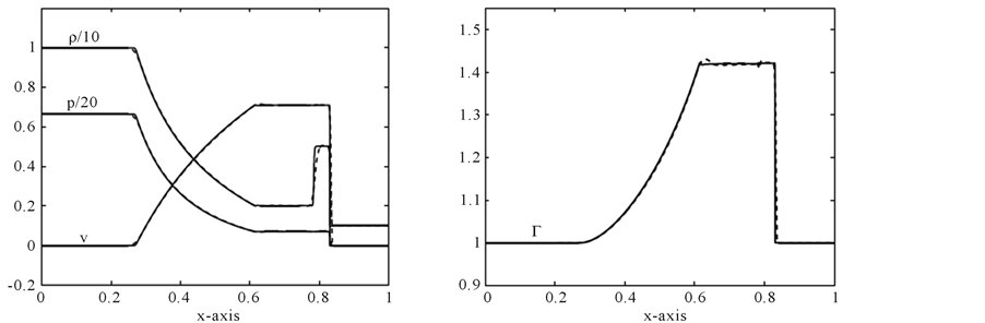

Figure 4. Comparison of problem 1 results at 400 mesh points (Dashed line) versus 4000 points (solid line) at t = 0.4.
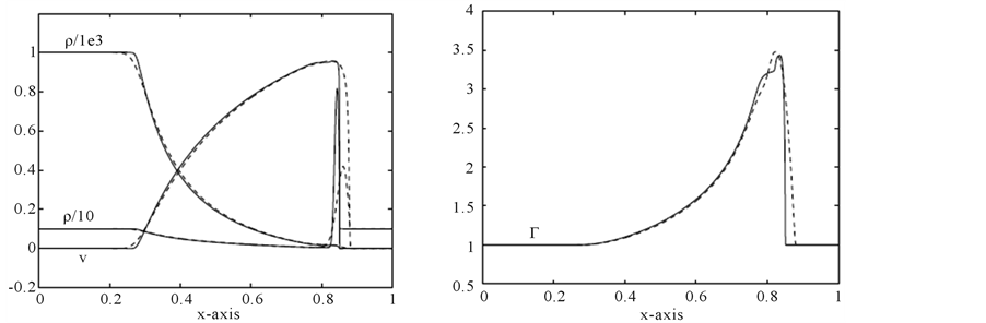

Figure 5. Comparison of problem 2 results at 400 mesh points (Dashed line) versus 4000 points (solid line) at t = 0.35.
 (i.e.,
 ), while jump in density in the shell reaches a value of 8.17.
Problem 3: A similar problem in non-relativistic case was solved by Quirk and Karni [26] . It consists of a  shock tube filled with air, where shock wave moves to the left. In the pre-shock wave stage, a bubble of Helium is set. The initial data are as follow

Here, the computational domain is . We compute the approximate solution of this problem with a grid of 400 mesh points at time
 . The reference solution is obtained at 3000 mesh points. The results are shown in Figure 6.
Problem 4: Cylindrical Explosion Problem:
Consider a square domain . The initial data are constant in two regions separated by a circle of radius 0.2 centered at
 . Inside the circle is helium with density 10.0 and pressure 13.33, while outside is air of density 1.0 and pressure equal to
  The velocities are zero everywhere. The specific heat ratios for helium and air are 1.67 and 1.4, while specific heats at constant volume are equal to 1 for both air and helium. The solution consists of a circular shock wave propagating outwards from the origin, followed by a circular contact discontinuity propagating in the same direction, and a circular rarefaction wave travelling towards the origin. The results are shown in Figure 7 for 400 mesh points at
 .
.
Problem 5: A  shock wave in air hits a Helium cylindrical bubble:
In this example, we introduce a single planar shock, moving in the air, with a cylindrical bubble of Helium. A schematic description of computational set-up is shown in Figure 8, where reflection boundary conditions are used on the upper and lower boundaries, while out flow boundary conditions on are used on the left and right boundaries. The bubble is assumed to be in both thermal and mechanical equilibrium with the surrounding air. The non-dimentionalized initial data are


Figure 6. Problem 3 results using 4000 points at t = 0.7.
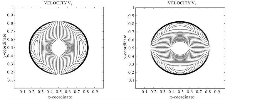
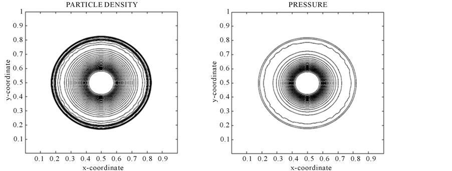
Figure 7. Problem 4 (cylinderical explosion) results using 400 × 400 mesh points at t = 0.15.
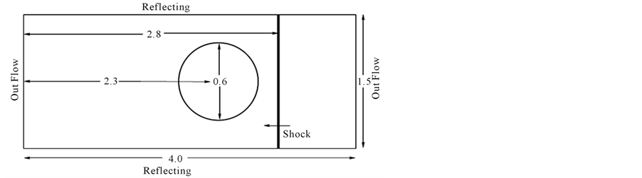
Figure 8. Sketch ok computational domain in problem 5.

Although the density in the bubble region is low, it is still stable. The results are shown in Figure 9.
Problem 6: Explosion in a box:
Here, we consider a helium gas with high pressure in a small box of sides length 0.2 at the center of a large box of unit length containing air. The outer box has reflecting walls. Initially the velocities are zero. The pressure of helium gas is equal 1000 and density equal to 1, while air has pressure 10 and density 1. The specific

Figure 9. Problem 5 (shock and helium bubble interaction) results at the different times.


Figure 10. Problem 6 (explosion in a box) results at different times.
heat ratios for helium and air are 1.67 and 1.4, while specific heats at constant volume are equal to 2.42 and 0.72, respectively. The results are shown in Figure 10.
6. Conclusion
A high-resolution staggered central scheme was applied to solve the relativistic multicomponent flow equations. The equilibrium states for each component are coupled in space and time to have a common temperature and velocity. Several case studies of the oneand two-dimensional flows were considered to validate the schemes. It was found that the suggested schemes have capability to resolve strong shocks without spurious oscillations. The schemes also guarantee the exact mass conservation for each component and the exact conservation of total momentum and energy in the whole particle system. The central schemes were found to be robust, reliable, compact and easy to implement for such complicated model equations.
NOTES
*Corresponding author.