Characterizing, Monitoring and Forecasting of Drought in Jordan River Basin ()
1. Introduction
Drought is a natural dynamic phenomenon that can inflict damages of disastrous proportions, which includes among other effects, the reduction of crop production and distressing the general population over the lack of water. Droughts occur in almost all climatic regions of the world with varying frequency, severity and duration but their impacts are aggravated in countries with limited water supply like Jordan. In contrast to aridity, which is a permanent feature of climate and is restricted to low rainfall areas, drought is a temporary aberration [1]. Many definitions of droughts have been adopted with reference to the components of the hydrological cycle and to the different impacts on water resources and ecosystems [2]. Reference [3] defined drought as a temporary imbalance of water availability consisting of a persistent lower than average precipitation of uncertain frequency, duration and severity, of unpredictable or extremely hard to predict occurrence, resulting in diminished water resources availability. Reference [4] introduced a broader and possibly more operational definition of drought as: the state of adverse and wide-spread hydrological, environmental social and economical impacts due to less than generally anticipated water resources quantities. Definitions are related to specific drought impacts and are generally classified into four categories which include: meteorological, hydrological, agricultural and socio-economic droughts [5].
For the purpose of this study, meteorological drought was adopted where precipitation is commonly used for drought analysis. Meteorological drought is defined as a lack of precipitation over a region for a period of time [6]. Droughts over a region can be characterized using different indices, which all use precipitation either singly or in combination with other meteorological elements, depending upon the type of requirements. Reference [6] discussed in a review paper a number of different indices that have been developed to quantify a drought, each with its own strengths and weaknesses. Drought indices evaluate the departure of climate variables in a given time interval (month, season or year) from the “normal” conditions and are used as monitoring tools and operational indicators for water managers. Drought indices can be either based on accessing the hydrological balance equation over different spatial and temporal scales such as the Palmer Drought Severity Index (PSDI) and Z indices [7], or on determining the precipitation deficits that trigger drought events such as the NOAA Drought Index (NDI) [8], and the Standardized Precipitation Index (SPI) [9].
The Palmer Drought Severity Index (PDSI), a wellknown index, is based on soil water balance algorithm that requires a comprehensive set of hydrological inputs [7]. The PSDI is a function of the soil water conditions of the recent and previous months. The Z index [7] shares the same algorithm with the PSDI but it is based on the soil water conditions of the recent month only. Thus, the Z index fluctuates more rapidly than the PSDI. It was found that the Z-index was the most appropriate for predicting crop yield in the Canadian prairies [10]. However, since its introduction by Reference [9], the SPI was widely used to measure the duration and severity of drought [4,11-16]. The NDI compares the historical mean of weekly precipitation and 8 weeks moving average of actual precipitation. If the normal precipitation exceeds the 8 weeks average by 60%, then drought conditions are considered until the precipitation deficit is eliminated. The SPI applies the precipitation probability to a standardized scale that consists of different levels of wet and drought conditions.
Reference [4] concluded that the SPI is appropriate for Mediterranean countries. Reference [17] found a linear relationship between vegetative conditions and the SPI. Similarly, Reference [18] reported that SPI calculated for 60 month period adequately predicts plant responses to drought.
Reference [11] results showed that the SPI12 (SPI estimated for 12 months period) and PSDI indicated similar drought trends for most of Europe. However, the SPI was favored over the PSDI because of the SPI’s standardized scale. The same consideration promoted Guttman to suggest the SPI as an alternative to the PSDI [19].
The Standardized Precipitation Index (SPI) is a tool which was developed primarily for defining and monitoring drought. It allows an analyst to determine the rarity of a drought at a given time scale (temporal resolution) of interest for any rainfall station with historical data. It can also be used to determine periods of anomalously wet events. The SPI is not a drought prediction tool. Reference [20] cited four advantages for the SPI scale; they are 1) the calculations for the SPI are relatively simple requiring only the precipitation as an input. 2) it can be calculated on different time scales suited for agricultural and hydrological applications 3) it is consistent measure of drought for any location and timescale because of the SPI’s standardized scale 4) it is not adversely affected by topography since it only depends on precipitation [20]. However, the SPI main disadvantage is that SPI calculation requires a precipitation monthly database of 30 years or longer.
Markov chains have been used for the stochastic characterization of drought [21]. An early warning system was developed by Reference [22] using Markov chain along with PSDI to probabilistically assess the severity, duration and return time of drought. Similarly, Paulo et al. (2005) and Paulo and Pereira (2007, 2008) applied Markov chain to the SPI analysis [13,23,24]. They characterized drought based on the probabilities of occurrence of different SPI’s drought classes, average duration of a particular drought, and short term prediction of drought based on the most probable SPI class 1 to 3 months ahead.
For drought forecasting, it is recommended to use time series analysis because it has two goals, modeling random mechanisms and predicting future series using historical data [25]. There are several methods that utilize historical record of rainfall in order to predict future trend. The most relevant would be the autoregressive integrated moving average (ARIMA) model which was introduced by Box-Jenkins in 1970 [26]. The ARIMA model, which is used in this paper, possesses many appealing features. It allows a researcher who has data only on past years (e.g., rainfall) to forecast future events without having to search for other related time series data such as temperature [27]. A comparison of six rainfall-runoff modeling approaches was conducted to simulate daily, monthly and annual flows in eight unregulated catchments in Australia [28]. It was concluded that a timeseries approach can provide adequate estimates of monthly and annual yields in the water resources of the catchments.
Jordan is very vulnerable to drought because of its limited water resources and its location at the edge of the arid zone and the desert of the Fertile Crescent. Water stress and scarcity are becoming a serious threat to the economic growth, social cohesion and political stability. Droughts are not predictable and are frequent due to the persistence of the Red Sea high pressure and jet stream path over the Gulf of Aqaba. When the jet stream moves north, a drought year is expected and a wet year is anticipated if the jet stream moves south [29]. Drought can certainly aggravate the water scarcity problem in Jordan and create severe crises. During summer, water rationings are enforced for domestic supply and the amount of water allocated for irrigation is usually reduced after successive droughts events. Therefore, Reference [30] proposed deficit irrigation strategies to cope with drought in Jordan. Drought research in Jordan is fragmented and limited but lacks the forecasting component. Few studies were conduced regarding drought identification and characterization in some localities in Jordan [27,31-33]. Reference [34] evaluated the SP1 and the NDI at several rainfall stations across Jordan. They found that severe drought tends to occur at large spatial scale. However, they did not have enough data to identify trends. This study covers the northern part of Jordan; namely the Jordanian part of the Jordan River Basin (JRB). The JRB includes major watersheds like the basins of the Yarmouk River, Zerqa River and other side wadies that flow into the River Jordan. The main problem in the JRB is the scarcity of water which is a result of the wide fluctuation in annual rainfall, population growth, urbanization and water quality deterioration. About 5.85 million people live in the basin compared to the country total population of 6.5 million [35]. Owing the importance of the area and in order to contribute to better water management and to help decision maker in water resources planning, this study was initiated aiming at 1) characterizing of drought and identifying its behavior using SPI, 2) studying the stochastic properties of the SPI at selected monitoring stations in Jordan, and 3) establishing a framework for drought forecasting in Jordan using Markov chains and ARIMA model.
2. Methodology
2.1. Precipitation Data and Trends Identification
Historical monthly precipitation records were obtained for Amman airport, Irbid, Mafraq and DeirAlla stations from the Jordan Meteorological Department (JMD). The four stations were selected to cover the whole area of the Jordanian part of Jordan River Basin. They have the longest historical records among other stations (Table 1). Table 1 also shows the location attributes and main statistical characteristics of the annual precipitation data collected from these stations. As shown in Figure 1, precipitation in Jordan starts on October and lasts till May, however, most precipitation occurs during December to March. The mean precipitation at Irbid was approximately 45% higher than the annual precipitation at Amman and DeirAlla stations. The monthly distribution was positively skewed at the four stations. However, the highest skewness was calculated for DeirAlla station. The MannWhitney test, available within the Change Point Model (cpm) package in R language, was applied for the all stations to ensure the homogeneity of the rainfall data.
2.2. Frequency Analysis
The return period (T) is a function of the probability distribution function F(XT) for wet condition, where rainfall is expected to equal or exceed a specific annual precipitation value. The relationship between F(XT) and T is expressed as:
 (1)
(1)
Whereas for drought condition, where total rainfall does not exceed a threshold level, the relationship becomes:
 (2)
(2)
2.3. Standardized Precipitation Index (SPI)
The SPI was used because of its suitability for Jordan and the Mediterranean region in general [4,34]. The Standardized Precipitation Index quantifies precipitation deficits by transforming the precipitation distribution into standardized normal distribution. The procedure for estimating the SPI has adequately discussed by previous researchers [11]. In this study, the built-in statistical functions

Table 1. Location attributes and statistical characteristics of the stations.

Figure 1. Normal monthly precipitation for Amman, Irbid, DeirAlla and Mafraq stations.
available in Microsoft EXCEL were utilized for the calculations of the SPI using three main steps, as follows:
1) Determining frequency distribution of the precipitation time series.
2) Fitting the precipitation distribution to the gamma cumulative distribution function (CDF).
3) Inversing the CDF from step 2 to cumulative normal distribution function to produce Gaussian CDF of zero mean and unity variance.
Reference [9] considered that an SPI value of <0 indicates a drought condition. The drought severity is categorized into four classes as mild (SPI ≤ 0 and SPI ≥ −0.99), moderate (SPI ≤ −1.00 and SPI ≥ −1.49), severe (SPI ≤ −1.50 and SPI ≥ −1.99) and extreme (SPI ≤ −2.00).
In this study, the SPI was calculated for the total annual precipitation. Also it was determined for the monthly cumulative rainfall; the total rainfall of the current month and the previous months, up to the months of October, November, December, January, February, March and April. The rationale behind using the cumulative amounts rather than the total amount for each month is that the precipitation in Jordan is scarce and the rainfall season is relatively short, therefore, an above average precipitation in a single month may prevent the onset of drought for the rest of the season; while a below average rainfall may create a drought condition that remains unrelieved to the end of the season. Thus, rendering the SPI values calculated from the total rainfall during a single month meaningless.
2.4. Markov Chain
Markov chain is a discrete stochastic process where the state (X) at a future time step (t + 1) is dependent on the current state Xt and independent of previous states, Xt − 1, Xt − 2,··· Xt−n. For a system of n states, X = {S1, S2,··· S3). The system can move from S1 to S2, S3··· Sn according to the transitional probabilities; p12, p13,··· p1n, or remain at state S1 with a transitional probability of p11. Thus, pij denote the transitional probabilities form Si to Sj. The transitional probabilities pij can be arranged in a matrix of n × n entries known as the transition matrix P, where the entries in each column represent the transition from any given state to the other state. Each entry is calculated from the number of transitions; nij, from a given state i to the next state j, thus:
 (3)
(3)
Hence:
 (4)
(4)
The transition matrix at any given time (Pt+n) is dependent on the transition matrix at the initial time (Pt) and the transition matrix of the previous time step (Pt+n−1) is:
 (5)
(5)
Markov chain becomes steady after several time steps. Thus, the stationary matrix π is:
 (6)
(6)
The stationary probabilities are independent of the previous state, therefore the entries in each row of π is equal to each other. Thus π is an Eigenvector of Pt provided that the Eigen value is 1 [36]. Noting that πj is the stationary probability for the state j then:
 (7)
(7)
Reference [36] presented persistence and recurrence time as two main descriptors of the Markov chain. Persistence is defined as the probability that the system will remain in the same state in following time step. Persistence probability (Pr) is expressed as:
 (8)
(8)
According to Reference [36] the recurrence time is the average time for the system to move from state j and then back again to state j. The recurrence time (tjj) is expressed as:
 (9)
(9)
Furthermore, Reference [23] considered the first passage time (tij) which is the time required for a system to move for the first time from state i to state j. They expressed tij as:
 (10)
(10)
2.5. Autoregressive Integrated Moving Average (ARIMA) Model
ARIMA is a time series forecasting model that combines the autoregressive (AR) and the moving average terms. The principle behind the autoregressive analysis is that the future value of the time series (yt) is dependent on the previous values of the time series. Thus, the autoregressive linear model is:
 (11)
(11)
where p is the order of the autoregressive model {e.g. AR (p)},  are the AR coefficients of the past time series values
  ,
,  is the random and independent error term, and C is a constant, usually assumed to be equaled to zero.
Solving the AR(p) system of Equation (11), e.g. using the Yule-Walker equations [37], would eliminate the error term because of the orthogonal characteristics of Equation (11). Therefore, the AR(p) predictions can be enhanced by including the moving average of past error or white noise in the time series:
 (12)
(12)
where q is the order of the moving average (MA) model {MA(q)} and  is the MA coefficients. The MA and AR terms can be combined in a single model in order to minimize the order of the AR model. The two can be combined to each other. Thus an ARIMA(p, q) is expressed as:
 (13)
(13)
The formulation of Equation (13) assumes a stationary time series, i.e. independent of initial conditions. However, many time series exhibits seasonal cycles and trends. Therefore, before using Equation (13) any cycles or trend should be removed in order to render the time series stationary, which can be accomplished by taking the difference between the current values yt and a lag from the previous values of the time series, yt-d, where d is the order or lag difference. Thus the order of ARIMA is (p, d, q) or ARIMA(p, d, q). The ARIMA model was fitted to SPI time series of Amman, Irbid, Mafraq and DeirAlla stations using the FORECAST package in the R programming language [38].
3. Results and Discussion
3.1. Exploratory Data Analysis
The 7-year moving average for the rainfall data collected from Amman station (data not shown) showed a slightly decreasing trend, however, the moving averages for the Mafraq and Irbid showed no increasing or decreasing trend, while the rainfall at DeirAlla stations demonstrated an increasing trend. Reference [32] statistically analyzed the historical rainfall record at Amman station (from 1922 to 2003). They suggested that stating the mid-1950s, there was an abrupt decline in the number of rainy days, but their analysis for the precipitation record at Mafraq station showed insignificant differences in the number of rainy days between the pre-1950 and post-1960 periods. The statistical analysis of the climatic record form six meteorological stations across Jordan showed trendless fluctuations in annual precipitation and maximum temperature, while the same results indicated an increasing trend of minimum temperature [33]. Reference [39] studied the structural characteristics of annual precipitation data for 13 meteorological stations distributed across Jordan and utilized the Isohyetal method to plot rainfall distribution. They employed a number of tests, such as consistency, randomness, best-fit distribution, and others in order to characterize the annual precipitation. There was no evidence of negative or positive precipitation trends at any station. However, these results cannot be directly compared with previous studies.
Using a 35 years of record (from 1970-2004), Reference [34] evaluated the SP1 and the Normalized Difference index at several rainfall stations across Jordan. They found that severe drought tends to occur at larger spatial scale. Using a Global Climate Model, they found a 10% average decrease in future rainfall for the year 2050. These results, however, were based on presumed climate change scenarios. Climate change is expected in the future, but the available research has not furnished a concrete evidence for an onset of climate change during the period of the historical record considered in this study.
The frequency analysis indicated a 2-year return period for near zero SPI values. This result is expected since the borderline between the wet and drought conditions corresponds with the average precipitation. It is possible to cope with an occasional occurrence of mild or moderate drought. However, it is evident that droughts occur frequently, which also implies the risk of successive droughts that occurred at least three time during the past 40 years, namely, from 1974 to 1977, from 1998 to 1990 and from 2004 to 2009 (Figure 2). In fact, three severe droughts were observed at Mafraq stations from 1958 to 1998 with an equal interval of 20 years. These droughts registered SPI values of −1.89, −1.52, and −1.79. The corresponding return periods were 34, 15.6 and 27.2 years respectively. Less dramatic, but more frequent severe drought were recorded at Amman station which has the longer historical record among the monitoring stations considered in this study. Five severe droughts were observed at Amman station with SPI values between −1.53 and −1.64 and a return period between 16 and 20 years. Similarly, the return period range
for severe drought at Irbid and DeirAlla stations were 16.5 to 39 years and 25 to 31 years; respectively. The extreme droughts were rare events with return periods between 70 and 93 years. Extreme droughts were not observed at DeirAlla station, while the number of extreme droughts observed at Amman, Irbidand Mafraq were 1 drought for each station, respectively.
3.2. Markov Chain
The results presented in Table 2 indicate equal occurrence probabilities for drought and wet conditions in any given year; irrespective, of the condition in the previous year due to the close proximity between the transitional and stationary probabilities. The yearly recurrence times calculated by Equation (1), and shown in Figure 3, were 1.7 and 1.8 years for the wet and drought conditions, respectively. Thus, two years is the average duration, or the time required, to return back from drought to wet condition. However, average drought duration greater than 1 and less than 2 years indicate that droughts can occur successively over several years. First order Markov

Table 2. First order Markov transitional and stationary probabilities (Wet and drought states were deduced from SPI values calculated on yearly basis).

Figure 3. The yearly recurrence time for wet (W) and drought (D) conditions.stations.
probabilities calculated on yearly basis are not sufficient to predict the succession of drought condition, especially that the yearly analysis is restricted to two conditions. Therefore, considering second order Markov transitional probabilities (Table 3) indicated that a drought at Amman station is more probable than the wet conditions after two successive wet or drought years. However, a drought is less likely than the wet condition if preceded by wet and drought sequence. For Irbid, DeirAlla and Mafraq stations the transitional probabilities for wet or drought condition are almost equal after two successive droughts. The other transitional probabilities for DeirAlla and Mafraq stations are similar to, but less pronounced, than transitional probabilities at Amman stations. At Irbid station the second order transitional probabilities showed that drought conditions should be expected after wet and drought sequence.
The monthly based Markov probabilities for three states, namely, wet, mild/moderate and severe/extreme droughts, presented in Table 4, gave better indications of the short term transition between similar and different conditions. The average drought duration was 4.5, 6, 6.5 and 5 months for the Amman, Irbid, DeirAlla and Mafraq stations, respectively as shown Figure 4. The importance of these determinations is that they are proximate with the actual length of the rainfall season. Therefore, drought occurring at the beginning of the seasonal will likely continue to the end of the season. The first expected passage time as shown in Figure 5 from any condition to wet

Figure 4. The monthly recurrence time for wet (W), mild/ moderate droughts (M) and severe/extreme droughts (E).

Figure 5. The expected passage times calculated using equation 7 for Amman, Irbid, Deir Alla stations. The expected transitions are: (W)(M): wet to mild/moderate drought, (W) (E): wet to severe/extreme drought, (M)(W): mild/moderate drought to wet, (M)(E): mild/moderate to severe/extreme drought, (E)(W): severe/extreme drought to wet, (E)(M): severe/extreme to mild/moderate drought.
or mild/moderately drought condition were between 4 to 6 months. However, the expected passage time from wet or mild/moderate drought to severe/extreme conditions was more variable among the four monitoring stations. At Amman station, approximately 16 to 20 months were required for the system to change from wet or mild/moderately drought to severe or extreme droughts. Whereas the first passage time to severe or extreme drought conditions was approximately 30 to 35 months at Irbid

Table 3. First order Markov transitional and stationary probabilities (Wet and drought states were deduced from SPI values calculated on monthly basis).

Table 4. Second order Markov transitional probabilities.
and DeirAlla stations and approximately 45 to 50 month at Mafraq stations. Thus, persistence of severe/extreme was less than the wet or mild/moderate drought. Also the severe or extreme droughts at Amman station were more frequent than the three other stations.
3.3. ARIMA Forecasting
ARIMA model of p = 20, d = 0 and q = 3 {ARIMA(20, 0, 3)} was fitted for Amman station. The model was calibrated using 48 years of the historical record, and validated on the remaining 38 years (Figure 6). The autocorrelation function (acf) plot of the calibration period (Figure 7) demonstrated a decline of the acf values after the first lag; thus indicating a quick convergence of the acf. Although the acf value never reached zero; however, allvalues lie within the 95% confidence intervals. Based on this interpretation of the acf function; it can be concluded that the SPI data series of Amman station is sta-

Figure 6. The comparison between the observed and simulated SPI values during the validation period for Amman station.

Figure 7. The autocorrelation function (acf) of the SPI time series at Amman station.
tionary and without evidence of seasonality. Therefore the order of d was set as zero.
The models were selected based on their performance during the calibration period, especially their ability to mimic the high and low values of the observed record. Therefore the selected orders of p and q were more than minimum orders inferred from the analysis of the partial autocorrelation function (pacf). However, Figure 8

Figure 8. Two partial autocorrelation functions (pacf) of ARIMA(3,0,0) and ARIMA (20,0,2) models, The two models were fitted to the SPI time series at Amman station.
shows a comparison between partial autocorrelation function (pacf) of the fitted model residuals and the residuals of ARIMA (3, 0, 0) and ARIMA (20, 0, 3). The pacf values indicate that an ARIMA model of a lower order sufficiently explain all the lags of the ARIMA (0, 0, 0). The SPI values predicted by ARIMA (3, 0, 0) were within −0.57 and 0.38 range. Such model falls short because of its inability to predict moderate to extreme drought events. On the other hand, the fitted model {ARIMA (20, 0, 3)} clearly improved the simulation results.
The model shown in Figure 6 predicted the exact SPI values of the droughts that occurred on 1983 (SPI = −0.9), 1985 (SPI = −1.53), 1993 (SPI = −1.26) and 2007 (SPI = −0.69). However, it overestimated or underestimated most of the drought or wet events. For some events it totally missed the prediction.For example, the model predicted that 1979/1980 was a drought season of an SPI of −1.0, where in reality it was an extremely wet season of an SPI value greater than 2.0. The model underestimated the extreme that drought of 1998/1999 and missed the prediction of the moderate droughts that occurred in two following season.
A closer look at the results showed that the model was successful in predicting the overall statistics with a given period at an annual scale. Using monthly time series, Momani (2009), found that the model was not appropriate to predict the exact monthly rainfall data. An intervention time series analysis could be used to forecast the peak value of rainfall.
At Amman station, the observed record during the validation period included 1 extreme drought event, and 2 severe, 3 moderate and 17 mild droughts events. In comparison, the model predicted 2 severe droughts, 4 moderate droughts and 14 mild droughts season. Similar results were reported in Jordan using graphical visual interpretation of depicted rainfall data of Amman and Irbid where 4 events of sever to moderate droughts for 20 year duration were found [29].
Similarly, ARIMA (24, 0, 2), ARIMA (20, 0, 2) and ARIMA (16, 0, 1) models were fitted for SPI time series at Irbid, Mafraq and DeirAlla stations. The ARIMA model performance at Irbid and Mafraq stations were similar to that of Amman station. At Mafraq station the model underestimated the extreme drought of 1997/1998 season, therefore the overall model predictions/observed record indicated 14/13 mild, 3/4 moderate and 0/1 extreme droughts as shown in Figure 9.
The ARIMA model at Irbid station, shown in Figure 10, predicted 8 mild drought events, in addition to 1 extreme and 1 moderate drought events, which compared well with that observed record that indicated 1 extreme, 10 mild and 2 moderate drought events. The ARIMA model for DeirAlla station (Figure 11) was inadequate possibly due to the relatively short observed record.

Figure 9. The comparison between the observed and simulated SPI values during the validation period for Mafraq station.
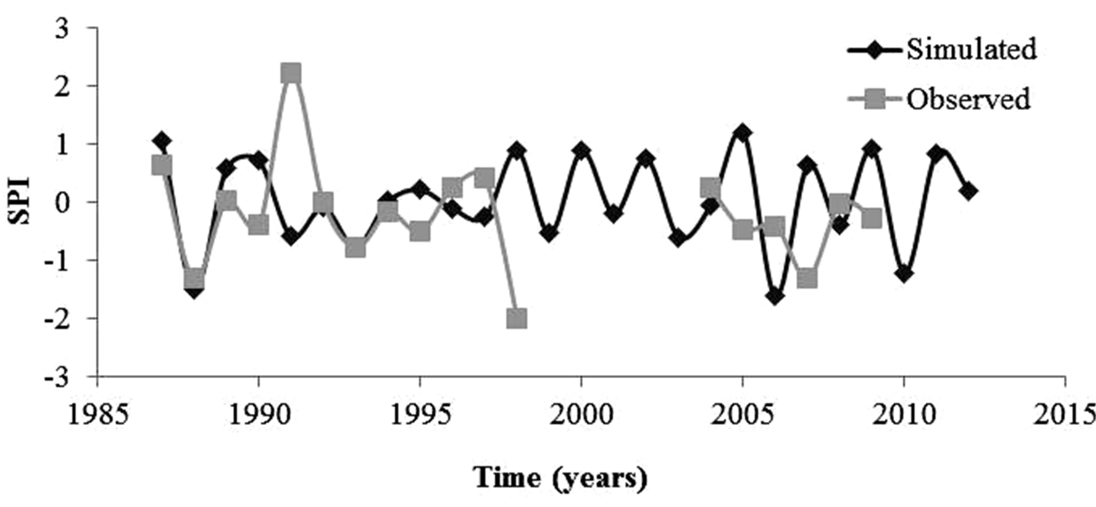
Figure 10. The comparison between the observed and simulated SPI values during the validation period for Irbid station.
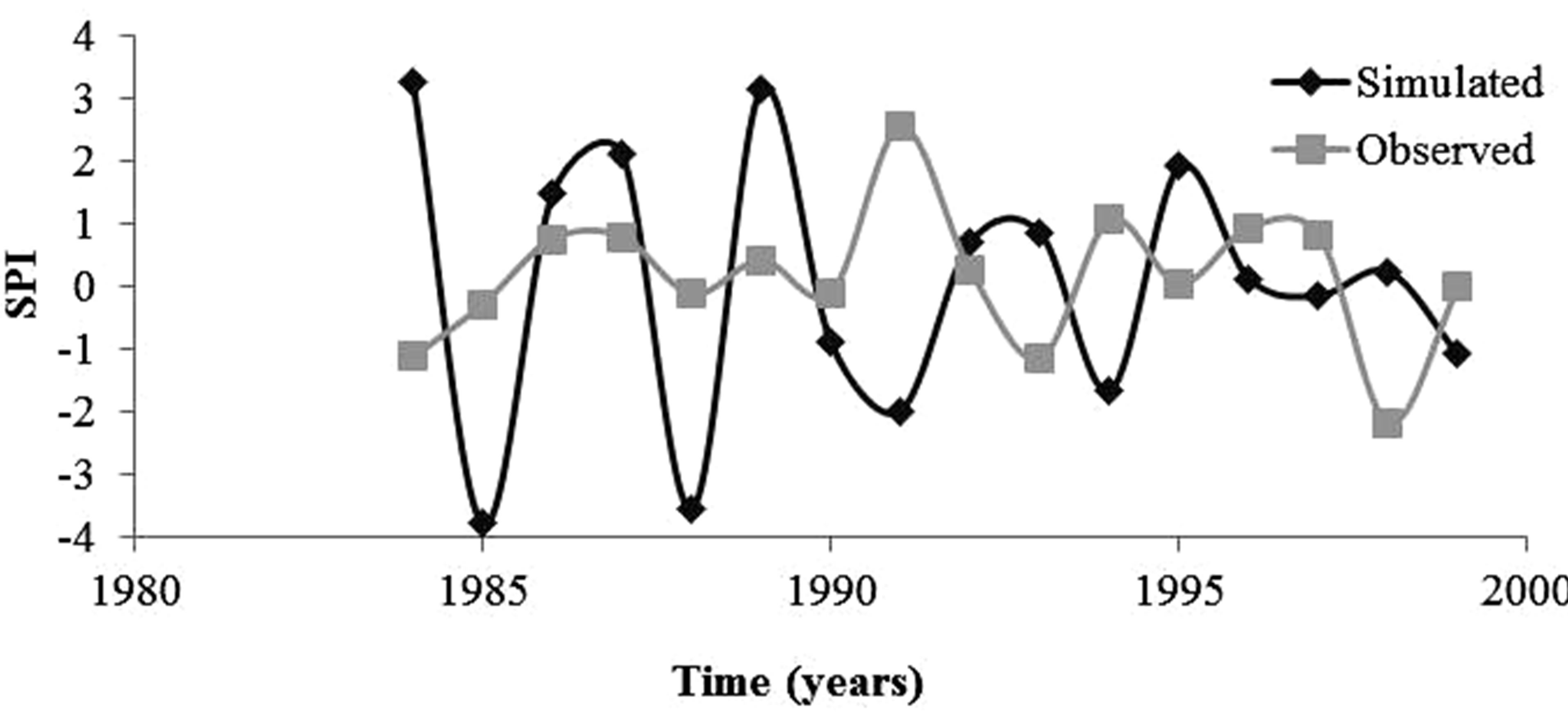
Figure 11. The comparison between the observed and simulated SPI values during the validation period for DeirAlla station.
4. Conclusions
Drought forecasting can be a challenging task since exact predictions of the SPI values are not possible using ARIMA model. By definition, Markov chain probabilities can give only the probable condition based on the antecedent condition of the one or two previous seasons. However, both methods can supplement each other in an important way and on three time scales levels.
Level 1: ARIMA models can be used as a long term (>10 years) forecasting tool of the future drought trends.
Level 2: Using the first and second order Markov probabilities to supplement the ARIMA predictions. For example, ARIMA models can predict a dry spells, however, interrupted by mildly wet seasons. Such results adjusted to more conservative prediction using the secondorder Markov probabilities indicate the drought will probably continue for the next season if it was preceded by two dry sequences.
Level 3: Early warning of developing droughts can be deduced form the monthly Markov transitional probabilities.
NOTES