Geostatistical Approach for Site Suitability Mapping of Degraded Mangrove Forest in the Mahakam Delta, Indonesia ()
1. Introduction
The Mahakam delta is located at the mouth of the Mahakam river on the east coast of Kalimantan, Indonesia. Including the distributary and interdistributary channels, the delta plain covers an area of 1500 km2. It was originally covered by dense mangrove, composed of mainly Avicennia, Sonneratia, Rhizophora, and Nypa species, and fresh water mangroves [1]. This ecosystem was disturbed since the introduction of shrimp farming. Human settlements also expanded because of the oil and gas exploration and exploitation, which attracted both workers and land speculators [2]. This ecological disturbance reached its peak during Asian economic crisis (1997- 2000) when shrimp price on the global market inflated to 4 - 5 times the normal level due to devaluation of Indonesian rupiah against international currency. This triggered mangrove forest conversion to ponds, involving heavy equipment, on a massive scale [3].
In 2001, 75% of the delta had been changed to ponds [4], which subsequently reduced to 52% in 2007, as reported by the Fishery and Oceanic Affairs Office of the Kutai Kartanegara District government [5]. Almost 90% of the Mahakam delta region belongs to the Indonesian Ministry of Forestry and is classified to be a production forest, however three other different government sectors lay claim to the management of the Mahakam delta: the Fishery Department, Interior Affairs Department, and the Environment Department [3]. Due to unclear management, laws and regulations, land use control of this area failed to be enforced.
Massive degradation of mangrove ecosystems has prompted a world-wide movement to plant new areas of mangroves [6]. Unfortunately, mangrove rehabilitation has often been carried out simply by planting mangrove seedlings, without adequate site assessment, or subsequent evaluation of the success of planting at the ecosystem level [7,8]. In this paper, we applied geostatistical and geographical information system (GIS) to generate site-suitability mapping for mangrove rehabilitation guidance in the Mahakam delta.
2. Materials and Methods
2.1. Study Area
The Mahakam delta is located between 117.30˚E - 117.62˚E and 0.49˚S - 0.82˚S (Figure 1). It comprises 46 sedimentation-formed islands [9]. For this study, we focused on areas (approximately 40,636 ha) where sample points were distributed relatively balance in term of spatial representation and therefore, data interpolation would give the best prediction.
2.2. Model Criteria and Flow Chart of the Study
In this study, we employed the technical guidance on mangrove plantation issued by Indonesian Ministry of Forestry in 2004. Geographical information system model was developed using the criteria presented in Table 1. ArcGIS 10 embedded geostatistical analysis tool was used to apply the model. Data normality were examined prior to geostatistics analysis. Geostatistical analysis tool was used to perform semivariogram analysis, ordinary kriging interpolation and subsequent cross-validation. Ordinary kriging interpolation produced a surface layer (continuous data) of all the data from our sample points. By superimposing all related surface layers, we can produce map of site suitability for mangrove rehabilitation over the entire area of the study. The major analysis steps used in this study were shown in Figure 2.
The physical data collected were soil texture (percentage of clay and sand fraction) and salinity. Tidal inundation data was derived from combination of a digital elevation model (DEM) and the 2009 tide table, obtained from the hydro-oceanographic division of the Indonesian navy. The digital elevation model was derived from the height points of the Mahakam delta topographic maps.
The tide table contained 12 months of hourly sea level rise predictions for a specific area. January, April, July and October were selected to represent the 2009 tidal prediction. We assumed each selected month would capture the seasonal effect of tidal dynamics in the area of interest. The East Kalimantan province is characterized by a tropical rain forest climate with a dry (May to September) and a wet (October to April) season [10]. The dry and wet seasons were represented by the months of July and January, respectively, while April and October represented the transitional months.

Figure 1. Location of Mahakam delta in the east coast of Borneo Island. The area sat the focus of this study are outlined by bold lines.

Table 1. Technical guidance of mangrove plantation in the forested areas of Indonesia.

Figure 2. The flow chart of the study, showing the major steps and the site-suitability map as the final result.
2.3. Semivariogram
A semivariogram is based on an assumption that properties of regions in proximity to one another are more alike than those farther away. In order to get a better interpolation result based on semivariogram analysis, we needed normally distributed data. The Shapiro-Wilk test was used to quantify the normality of the data. We used the BoxCox and logarithmic transformation to normalize the data. After that, we used the semivariogram analysis to quantify the spatial relationship between the sample points. The semivariogram symbolized by g(h) is the average variance between observations separated by a distance h. It was computed using formula:
 (1)
(1)
where γ(h) is the experimental semivariogram value at a distance h; N(h) is number of sample value pairs within distance h; and z(xi), z(xi + h) are the sample values at two points separated by distance h. All pairs of points separated by distance h (lagh) were used to calculate the experimental semivariogram.
The semivariogram parameters are the range, total sill and nugget ratio. The total sill is the sum of the sill and nugget, while the nugget ratio is the ratio of the nugget to the total sill [11]. Lag is the distance between two pairs data; the sill is the maximum level of γ(h); the range is the point on the h axis where γ(h) reaches a maximum [12]. The experimental semivariogram will be fitted using a mathematical model used for interpolation. There are many models available, but the most acceptable ones for continuous variables would be spherical, exponential, Gaussian or combinations of these models [12]. In this study, we used a Gaussian model with a small range and sill value, which means this model predicted smaller data variability compared to the spherical and exponential models.
2.4. Kriging Interpolation
We applied Kriging interpolation to clay, sand, salinity and height point data following the semivariogram investigation. Reference [13] discovered that kriging interpolation was better suited for prediction and mapping of the distribution of chemical soil properties while reference [14] found that kriging interpolation had successfully explained soil properties. We chose widely used ordinary kriging interpolation to generate the model, assuming the absence of non-linear trends and focusing only on the spatially correlated component [15].
The characteristics of an interpolated surface layer can be controlled by limiting the input points used in the calculation of the output cell values. Specifying the maximum and minimum number of points to be sampled will return the points closest to the output cell location, until the maximum number is reached. This number is then used in calculating output values. In this study, we used a combination of maximum and minimum number of neighboring points to be 5 and 2, respectively. Another method to control the interpolated surface is by defining either a circular or elliptical model to enclose the points that are used to predict output cell values. Furthermore, these circular or elliptical models could be divided into sectors. We used a circular model split by a diagonal cross section (4 sectors with a 45˚ offset) for calculating output cell values.
Surface layer-based interpolation data were classified according to criteria shown in Table 1. To divide the surface layer into classes (suitable, moderate or not suitable) especially for clay and sand data, we used Jenks natural breaks provided in most of GIS softwares. Salinity data was divided into two classes: 0 - 10 ppt (part per thousand) and 10 - 30 ppt. From DEM data, we defined three classes of tidal inundation based on the number of inudation days in a month: 1) more than 20 days in a month; 2) between 10 - 20 days; and 3) less than 10 days in a month.
2.5. Validation
Cross validation of sample points was used to measure the model accuracy. The following statistics were used:
root mean square (RMS), which measured error size sensitive to outliers [16], and standardized RMS [15]. RMS was calculated using the following formula:
 (2)
(2)
By dividing RMS with standard error then standardized RMS would be obtained. Here the variables are defined as follows:
Zi,act = the known value at point iZi,est = the estimated value at point in = the number of points.
3. Results
3.1. Normalizing Data
The normality test using Shapiro-Wilk method indicated that our data was not normally distributed (Table 2). Therefore, data normalization was imperative prior to kriging interpolation. Only clay data appeared to be normally distributed, since its p-value was close to 0.05. We performed a standard statistical calculation and found that sand, salinity, and height data exhibited higher variation than the clay data. Coincidently, the high variation was related to the p-value of Shapiro-Wilk.
We used the Box-Cox transformation for all data, except clay, which was transformed using a logarithmic method. The Box-Cox improved the efficacy of normalizing and variance, equalizing for both positivelyand negatively-skewed variables [17].
3.2. Producing the Tidal Inundation Map
We analyzed 4 monthly tide tables and found that the tide rose somewhere between 0 - 3 m. The lowest altitude area was assumed to be inundated in longer period than higher altitude area. We summed up days exceeding a certain tidal height interval (0.1 m) and determined as inundation period starts from 0 m above sea level. Following tidal inundation classes (Table 1), we obtained specific height thresholds to separate the classes that is 1.1 and 1.6 m of altitude (Figure 3).
3.3. Semivariogram and Kriging Interpolation Analysis
Lag size and the number of lags are two parameters that

Table 2. Descriptive statistics of the four types of data.
contribute to the number of pair points generated in a semivariogram graph. The number of lags was set to 12, which is the default value set by the geostatistical analysis tool. From Figure 4, we found that variation in the sand data was confirmed to be the highest one, as indicated by the nugget value equal to 16.024, as shown in Table 3. However, we also found that salinity data need a longer distance to reach the sill value (nearly 45 km).

Figure 3. The number of inundation days for each of the height levels summarized from tide table.
Kriging interpolation accuracy was inspected through RMS and standardized RMS. However we could not compared RMS values, since the units were different. From the standardized RMS value, we found that clay and height data underestimated the variability of prediction (standardized RMS < 1), while sand and salinity would be overestimated (standardized RMS > 1).
3.4. Surface Classification Using GIS
Kriging interpolation produced surface layers, as shown in Figure 5. Clay fraction data after interpolation ranged between 7.4% and 52.8%. Two clay classes were defined using the Jenks natural break. Moderate class for clay was within the range 7.4% - 28.2%, while the suitable class was 28.2% - 52.8%. Sand data after interpolation ranged between 5.5% and 76.0%. Using similar method, three classes were generated and classified as: not suitable (5.5% - 25.6%), moderate (25.6% - 46.8%) and suitable (46.8% - 76.0%). Digital elevation model was classified as 1) elevation less than 1.1 m, which would be inundated more than 20 days a month; 2) elevation higher than 1.6 m, which would be inundated less than 10 days in a month; and 3) elevation ranging between 1.1 and 1.6 m, which would be inundated within 10 - 20 days in a month.
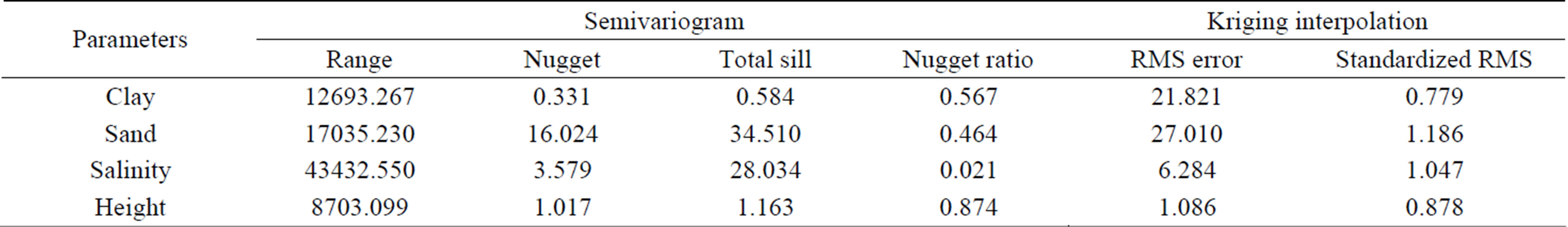
Table 3. Semivariogram parameters for each data with RMS and standardized RMS values after kriging interpolation.
According to Table 1, there are ten unique zones of mangrove species. Some of the species shared similar site characteristics, such as Rhizophora mucronata and R. apiculata or Bruguiera parviflora and B. sexangula. The GIS-based overlay of whole surface layers produced 12 unique sites with different combination of all data. A site-suitability map of mangrove species was generated corresponding to criteria in Table 1. The results showed that three site zones were not represented in any GISunique sites, i.e. zone B (Rhizophora stylosa and Sonneratia alba), G (Lumnitzera racemosa), and H (Cerbera manghas). The final map of site suitability of mangrove species is presented in Figure 6.
4. Discussion
4.1. Geostatistical Analysis
Reference [18] explained that non-normal data is actually common in geostatistical data, especially if the observed data is discrete, i.e. ppm, percentages of grade, etc. Moreover, reference [19] showed that in the case of soils, they naturally form in different depositional environments; therefore, their physical properties vary from point to point (in the horizontal as well as vertical plane). Thus, we assumed the existing variation of our data were natural.
Semivariogram graphs shown in Figure 3 describe the relation of semivariance value (y-axis) and distances (xaxis). All data (clay, sand, salinity and height) seemed to follow the theoretical assumption of semivariogram, where points that are close to each other are expected to have small variance, and points that area farther apart are expected to have higher variance [15].
As shown in Table 3, the highest value for the sill element was that of sand, which means that the variance among the sand sample point data is greater than for other data. However, semivariogram measuring salinity showed that more than 43 km were needed to get variance to decrease, while clay had the smallest such distance. Sand data had the highest nugget value, which might indicate the highest measurement errors. Nevertheless, all semivariogram graphs showed a natural experimental omnivariogram.
Clay data had RMS error equal to 21.82%, which was smaller than sand with 27.01%. While salinity had RMS error of 6.28 ppt and height error 1.09 m. Standardized RMS value had juxtaposed our data into 2 groups (clay with height and sand with salinity) respecting to the estimation of the variability of the predictions. However, according to reference [20], statistical value is not the only source of assessing the interpolation quality; we also need to carefully study the visual quality of the surface model generated by kriging interpolation to detect distinct spatial patterns and visual faithfulness.
4.2. Analysis of Spatial Data Interpolation
We compiled 66 sample points for soil texture and 67 sample points for salinity, both onand off-shore. Samples were not spread evenly across the area but rather clumped in the southern part and missing in the central part. As a result, the study only focused on some parts of the Mahakam delta, which would have the best interpolation results. The interpolation process ignored the distributary channel and assumed that the topographic features in the delta plain were negligible [21].
Soil type in the Mahakam delta is loamy, varying from silt loam to clay loam, except for the coastline which is loam with sand [2]. According to Figure 5, we found consistency in this fact, whereas higher clay concentration dominate over the area of study. The sand fraction concentration is located at the outer delta, while clay mostly deposits in the center of delta, straight to the Mahakam river flow discharge direction. Although pond construction altered land, however, soil texture was assumed to remain fairly constant and was unchanged by management practices [22,23]. A suitable class for clay and sand means that both fractions have a high percentage. A high concentration of clay dominated 95% of the study area. A species preference for high percentage of clay implies that species was intolerant to the high percentage of sand and vice versa.
Salinity also showed a natural distribution, where higher concentration situated in the outer delta rather than the inner delta. Salinity data is one of the sea water environmental factors that would spread gently and smoothly, especially in the estuary region. The total salinity range of the open ocean is about 30 - 40 parts per thousand (or ‰) while salinity in coastal estuaries can be much lower [24].
Altitude ranged from 0 - 4 m above sea level, with an average 2.26 m. A digital elevation model was generated

Figure 6. Site suitability map of our study sites generated using geostatistical analysis and GIS operations.
by kriging interpolation. The interpolation produced continuous elevation, ranging from 0 to 4.64 m. Normally higher elevation area are located in the inner delta, but interpolation found another high elevation area in the outer delta, near the coastline (Figure 5(d)). This area used to be an agricultural spot planted with coconut trees. However, during the introduction of shrimp pond, this area was also converted. The construction of ponds changed the terrain to flat.
4.3. Site Suitability Mapping
Site suitability map as an output of spatial combination of four physical characteristics showed that theoretically 10 mangrove species were suitable for planting in the barren area or abandoned ponds. We calculated that 50.25% of the study area was suitable for Avicennia sp. and the other 42.22% suitable for Nypa fruticans. These two species occupied 92.69% of the study area. Another 7.14% was shared among Sonneratia caseolaris, Rhizophora mucronata, R. apiculata, Xylocarpus granatum and Heritiera littoralis. Only 0.16% would be suitable for Bruguiera species, which is known to prefer to grow at the boundary between mangroves and the coastal ecosystem, in the middle and upper inundation areas [25]. These results were consistent with the mangrove zoning, where Avicennia sp. is naturally found adjacent to the sea, together with Sonneratia species [26]. Meanwhile, Nypa fruticans seemed suitable to areas behind Avicennia sp., where brackish to almost freshwater streams exist and tidal effects decline.
Regarding to the rehabilitation efforts, site suitability map will assist the authority to prepare and implement rehabilitation strategy in this area. However, further studies are needed to validate this conceptual model by establishing small-scale demonstration plots and planting various mangrove species, to periodically compare their growth and mortality. Even though Avicennia sp. and Nypa fruticans seem suitable for about 92% of the total study area; it does not mean that other species will not survive if planted. Reference [26] emphasized that overlapping between species or zones occurred at many sites.
4.4. Site Suitability Mapping
Reference [27] reported that Total E&P Indonesia (company developing oil and gas) have planted more than 3 million mangrove trees on cleared areas, mainly along the pipeline distributional network. However, on a broader scale, mangrove rehabilitation in the Mahakam delta is still a minor project, due to unclear land ownership. Most of the ponds are effectively “owned” by the people operating them, so that plantation programs cannot be implemented in all necessary locations. Rehabilitation projects needs to be prepared carefully otherwise they will trigger social conflict. As a top priority, reference [2] suggested restoring mangroves in the areas that are incompatible with pond production due to poor soil quality or required for coastal protection.
In the case of the Mahakam delta region, a social approach for rehabilitation of the “occupied” land is a prerequisite to any such rehabilitation program. It is complicated by a number of factors, including the lack of clarity in land status, which, in theory, mostly belongs to the state, as well as the claims of the local people. Although these claims are illegal, it is impossible to restore the land without compensation to its current users; this is the main obstacle for rehabilitation programs in the region. Spending government fund for compensation is currently only permitted for private, not public, land. Recently, some small-scale silvofishery projects funded by a private company and an NGO had been introduced to this site in the last 3 - 4 years. However, most of the degraded areas remain barren and need immediate action to bring back the ecological function of mangrove forests for future generations.
5. Conclusion
Our study demonstrated an original approach to producing a site-suitability map of mangrove for rehabilitation purposes by combining 4 factors (clay, sand, salinity and height) using geostatistics. We proposed a new approach to making tidal inundation maps. Based on this study, we suggest height points linked with tide tables to produce tidal inundation maps. Statistical values and visual inspection of surface layers as a result of kriging interpolation yielded consistent results therefore, we assumed that interpolation processes have been carried out appropriately.
6. Acknowledgements
We would like to appreciate and thank Total E&P Indonesia, Dr. Iwan Suyatna from the Faculty of Fishery and Marine Sciences, University of Mulawarman, and the Faculty of Forestry, University of Mulawarman, for kind support in providing various data related to this study