1. Introduction
A limit cycle, which is represented by an isolated closed trajectory in the phase plane, describes a phenomenon of oscillation that is widely observed and studied in various research fields such as electrical circuits and control theory [1], chemistry and medicine [2,3], ecological systems [4], human population [5], etc. Some research focuses on the analysis of properties of limit cycles such as stability and period [6,7]. Besides, a variety of theorems on detecting the existence and the number of limit cycles are also developed by many researchers [8-10]. While, beyond these topics, identification of limit cycles remains to be a difficult problem. In previous research, different methods and theories are established for constructing approximated limit cycles (e.g., via harmonic balance, power series) [11,12]. However, little development is achieved in respect of identifying exact analytical formulas of limit cycles for a general system or a family of equations.
In this paper, we propose a new framework for identifying the limit cycles of polynomial systems, inspired by the latest innovation in multivariate polynomial representation and roots finding by formulating the polynomial equations via Macaulay matrices [13,14], thereby turning the problem into an eigenvalue computation problem.
In the proposed framework, an equation of semi-invariant that captures limit cycles is formulated via linear algebraic representation, by assuming that the limit cycle is represented as a multivariate polynomial. Afterwards, a two-level Macaulay matrix approach is applied to solve the set of equations. First, the semi-invariant equation is reformulated by representing multivariate polynomials and their multiplications with coefficient vectors and monomial vectors, based on the concept of Macaulay matrix. A set of polynomial equations are then constructed with respect to the coefficients of the limit cycle, whose roots are found through eigenvalue computation. This framework has a general efficacy for polynomial systems of arbitrary orders and dimensions.
Moreover, our method is applicable not only to systems with polynomial limit cycles, but also to systems with non-polynomial limit cycles containing common terms such as exponential and logarithmic kernels. We achieved this by exploring and flexibly using immersion, a method for eliminating non-polynomial terms, to enlarge the scope of application. Therefore, the proposed framework provides an innovative method for limit cycle identification for polynomial systems.
The remainder of this paper is organised as follows. The concepts related to limit cycles and polynomials are introduced in Section 2. Then we present in Section 3 a two-level approach based on Macaulay matrix to solve for the limit cycle. In Section 4, we review the concept of immersion and its novel use to extend our framework to non-polynomial limit cycle identification. Section 5 demonstrates the entire procedure with examples. Finally, Section 6 concludes this paper.
2. Theoretical Background
2.1. Stable Limit Cycles and Semi-Invariants
Given an autonomous system,
 (1)
(1)
where  are polynomials in the variables
  . If one of its trajectories traces out an isolated closed curve, the curve is called the limit cycle of the system. If all trajectories in its neighbourhood spiral towards the limit cycle (outer trajectories shrink and inner trajectories spread) as shown in Figure 1(a), then it is a stable limit cycle.
The LaSalle’s theorem in particular [15] can be used to capture stable limit cycles:
LaSalle’s Theorem: Let  be a compact set, positively invariant with respect to system (1). Let
  be a continuously differentiable function such that
  in
in . Let
. Let  be the set of every point in
  where
where . Let
. Let  be the largest invariant set contained in
 . Then every solution starting in
  approaches
  as
as .
.
Suppose the system has a polynomial limit cycle . Define
 . To achieve a stable limit cycle, set
  according to the LaSalle’s theorem. Then,
 . Hence we have
  and
and . For
. For  to be continuous, we have
 , or
, or  divides
 . For system in (1),
 . By the definition of directional derivatives
 , we have
 (2)
(2)
with h, the quotient of  divided by
 , being a polynomial as well. Such
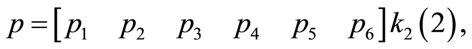
  that satisfies (2) is studied in a variety of topics, with names such as semi-invariants, second integrals, eigenpolynomials etc. [16]. In this paper, the semi-invariant associated with system (1) plays the role of limit cycle. For (2), notice that
  results in a special case that
 . Such
  is known as a first


Figure 1. Stable limit cycle and neutrally-stable limit cycle: (a) plots a stable limit cycle that attracts nearby trajectories; (b) plots neutrally stable limit cycles consisting of infinite closed trajectories (only part of them are plotted).
integral, which expresses a specific kind of stable limit cycles, the neutrally-stable limit cycles. In this case, the system has infinite non-isolated closed trajectories as shown in Figure 1(b).
2.2. Representation of Multivariate Polynomials
Any multivariate polynomial can be represented with a coefficient vector multiplied by a vector containing all monomials up to a certain degree. Suppose we have a general bivariate polynomial of degree two,

It can be expressed as,
where 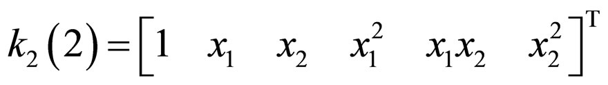 consists of all monomials of variables
  up to degree two. Similarly, in the rest of the paper, vector containing all monomials of
  variables
  up to degree
  is noted by
 . Furthermore, if
  is multiplied by a monomial, the result can be expressed as a “shifted’’ coefficient vector of
  multiplied by the
  vector of extended order. For example

Now, consider the multiplication of p and another general polynomial q. Since q can be regarded as a linear combination of monomials, according to the representation above, it can be seen that the coefficient vector of  is also a linear combination of coefficient vectors of p multiplied by each monomials in q. By stacking these coefficient vectors, a truncated Macaulay matrix can be constructed, with coefficient vectors of p and its shifted versions as rows. If
 , then the multiplication of p and q can be expressed as,

3. Two-Level Macaulay Matrix Approach
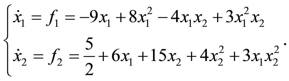
In this section, we present how the two-level Macaulay matrix approach works on finding limit cycles of polynomial form. The entire procedure is divided into two stages. First, with the assumption that the limit cycle is a polynomial of a certain degree, all polynomials and their operations in (2) are represented in the way described in Section 2.2. By equating the coefficient vectors on both sides of (2), a set of polynomial equations are set up whose variables are coefficients of all unknown polynomials in the equation, including those of the limit cycle. Therefore it is sufficient to obtain the accurate expression of the limit cycle by solving those polynomial equations. Generally, a polynomial limit cycle can be of any order. Therefore, with initial trial of a certain order, we iteratively increase the order of the limit cycle. At each iteration the solved coefficients indicate the termination: the recursion stops when a set of valid coefficients of a limit cycle are obtained. We illustrate the idea through a walkthrough example. Given a third-order bivariate polynomial system with a polynomial limit cycle of unknown order,
 (3)
(3)
by assuming the limit cycle is of a certain degree, say degree 2, the general form of such limit cycle is  . By comparing the degree on both sides, the degree of cofactor h,
 . Therefore, by utilizing the notion in Section 2.2,

Therefore, the L.H.S. of (2) becomes

Similarly, R.H.S. becomes

The corresponding coefficients of each monomial in  on both sides must be equal, which generates a set of 15 polynomial equations in 12 variables.
 (4)
(4)
Notice that further investigation based on observation of the numerical simulated limit cycle makes the equations more compact: firstly, the origin does not lie on the limit cycle, which forces  nonzero. We might as well set
  since the limit cycle
  still holds; moreover, the limit cycle has two intersection points on each of
  and
and  axis, indicating that
 has two roots of
  w.r.t.
  (same for
  w.r.t.
 ). Therefore
  and
and  are both nonzero. Accordingly, it reduces (4) to a set of 9 equations in 7 variables, as below,
 (5)
(5)
Next, these polynomial equations are manipulated by putting coefficients in a Macaulay matrix and unknowns in a monomial vector, such that the problem is converted to a linear algebraic one. Given a polynomial system , of degree
  and in
  variables
 , the approach at this stage is accomplished in three steps [13,17]:
1. , a Macaulay matrix of degree
  in
in  variables
 , is constructed with
 (6)
(6)
where for each , monomials from degree 0 up to
  are multiplied,
 .
.  contains the coefficients of (6). In other word, expressions in (6) can be represented by
 .
.
2. By first performing a left-right permutation, then regulating  into reduced row echelon form, the distinct leading monomials in the row space of
  are observed. These monomials of
  are denoted by
 . The vector space spanned by
 , and its complement spanned by the remaining monomials are denoted by
  and
and , respectively. Then those monomials span
  are defined as normal set
 . The decomposition of monomial basis into
  and
and  is called canonical decomposition, implemented by principal angle computation through SVD. Furthermore, the reduced monomials are defined to be the smallest subset that divides
 , denoted by
 . That is, for each monomial in
 , there exists a monomial in
  that divides it. Then the reduced normal set
  is the normal set corresponding to the canonical decomposition implied by
 .
.
Starting from the initial , the degree of
  is stepped up. The Macaulay matrix of a proper degree
  is found when the corresponding
  stops changing as
  increases. To eliminate roots at infinity, the reduced Macaulay matrix
  is constructed with
 .
.
3. Once  is constructed, the affine roots are retrieved from the canonical nullspace
  of
of . Whereas K is not directly available, the basis of the nullspace, Z is first computed by SVD. Then K is proposed to be obtained by
  where V is a nonsingular matrix. Let
  and
and  be two row selection matrices, and
  a freely chosen diagonal matrix, such that
 . Replacing K with ZV on both sides,
 . Alternatively,
 (7)
(7)
where  is the pseudo-inverse of
  since
since  is not necessarily square. Therefore, V is obtained by computing the eigenvectors of
 . Once V is available, K is solved with
 . With first element normalized to 1, columns of K represent monomial vectors containing monomials valued at affine roots of the system. Hence, all affine roots are retrieved.
As described above, the two-level Macaulay matrix approach obtains a set of possible coefficients of the limit cycle. This process iterates by increasing the order of the limit cycle and inspecting the validity of the coefficients solved at each iteration, until a valid limit cycle is obtained, if there exists one. For equations in (5), initially  of size
  is constructed. By inspecting
 , the Macaulay matrix sufficient for solving affine roots is
 . Through eigenvalue computation, the affine root is obtained as
 .
.
Therefore, the limit cycle is .
.
4. Immersion
In this section, we extend our framework to non-polynomial systems or non-polynomial limit cycles by immersion. Immersion was introduced in control theory for decades [18]. The main idea is to eliminate the non-polynomial kernels in nonlinear systems by adding new state variables. Through immersion, the original system is transformed into a polynomial system with more states. Therefore, our framework is also applicable to non-polynomial systems that are convertible via immersion. Moreover, by flexible use of the idea of immersion, we can similarly transform a non-polynomial limit cycle into a polynomial one by eliminating its non-polynomial terms. For a limit cycle with common nonlinear terms, e.g., exponential or logarithmic nonlinearity, by defining new states to replace those terms, we get a new system with a polynomial limit cycle. The new system has more states, yet transforming the problem into where our framework is applicable. This enlarges a lot the scope of polynomial systems compatible with our proposed method. The Lotka-Volterra (LV) equations, which are widely used for describing behaviors of biological systems, is a bivariate polynomial system as below,
 (8)
(8)
with its limit cycle known to be
 . The Macaulay matrix approach unsurprisingly fails for LV equations since the assumption of a polynomial limit cycle never holds due to the existence of logarithms. However, by utilizing immersion, the framework regains efficacy. Defining two new states
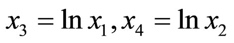 , and taking Lie derivatives
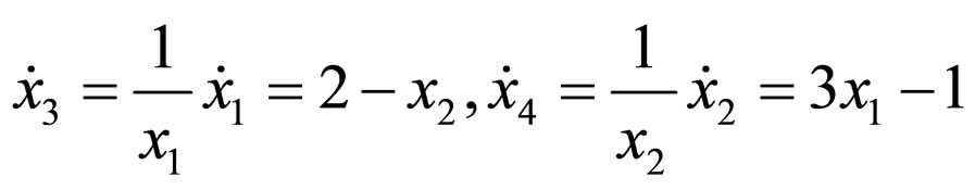 , the LV equations are extended to a four-state polynomial system
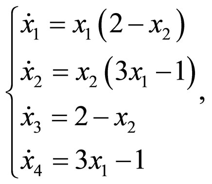 (9)
(9)
with limit cycle now being , a polynomial. Therefore, the extended system falls into the scope of our framework. Inputting the extended equations through the two-level Macaulay matrix approach in Section 3, we have
 , i.e.,
 . Substituting
 , the limit cycle
 is retrieved. Substituting back to (2), we have
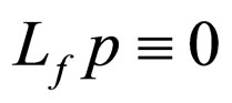 . Therefore
 expresses neutrally-stable limit cycles as mentioned in Section 2.1.
5. Examples
In this section, we illustrate the feasibility and applicability of the technique presented in the previous sections with examples.
5.1. A Third-Order Bivariate Polynomial System
First we study the planar cubic system
 (10)
(10)
The semi-invariant equation is
 (11)
(11)
Initially, p is assumed to be a first-order polynomial. Through the procedure, the order of p is increased iteratively until a valid limit cycle is obtained. Employing the first stage of the Macaulay matrix approach, the identification of the first-order, second-order and third-order limit cycle  is converted to solving for systems of 10, 15 and 21 equations, respectively. At the second stage, only trivial solutions are found for the above cases, i.e. either
  or
or  is a constant. These solutions do not represent a valid limit cycle. Now, assume the limit cycle is of order 4. Equation (11) is formulated into a set of 28 equations in 21 variables,
 (12)
(12)
where  represents the coefficient of
  in the limit cycle. Numerical simulation of (10) implies that the origin does not lie on the limit cycle, which indicates a nonzero
 . Therefore, we might as well set
  to eliminate the trivial solutions
  with arbitrary
 . Then, (12) becomes,
 (13)
(13)
Such modification does not reduce the number of equations. However it makes the Macaulay matrix approach feasible. After applying the Macaulay matrix approach, the affine roots of (13) is found as

with remaining coefficients all being 0. Therefore, a valid limit cycle of degree 4 is obtained,
 (14)
(14)
Figure 2 compares the level curve
 with a simulated trajectory of system (10). It verifies that the obtained limit cycle in (14) does capture the limit cycle of the system.
5.2. A Bivariate Non-Polynomial System with Exponentials
Given a non-polynomial system,
 (15)
(15)
First, immersion is applied to transform (15) to a polynomial system. Notice that the non-polynomial non-linearity is caused by . One may guess that the limit cycles of (15) also contain such nonlinearity. Therefore, define
  and add the Lie derivative
 to (15). We have,
 (16)
(16)
Thus, a forth-order polynomial system in variables  is obtained via immersion and it falls into the scope of the framework. Similarly to Section 1.5.1, by assuming (16) has a multivariate polynomial limit cycle
 , the Macaulay matrix approach is iterated by increasing the degree of
 . A valid affine root is found for
  of degree four. The limit cycle is

Figure 2. Plots of (14) and a simulated trajectory of (10) spiraling towards the limit cycle.
identified to be
 .
.
Substituting , the limit cycle for the original system (1.15) is retrieved,
 (1.17)
The level curve (17) and the numerical simulation of trajectories of (15) are plotted in Figure 3, showing that the identified limit cycle attracts nearby trajectories as expected.
6. Conclusion
This paper has presented a new framework for finding multivariate limit cycles for polynomial systems. This framework employs a two-level Macaulay matrix approach to convert the limit cycle identification to a problem of solving multivariate polynomial equations, and finds the roots with linear algebra and eigenvalue computation. The procedure iterates by increasing the degree of the polynomial limit cycle until a valid limit cycle is obtained. Furthermore, the scope of the framework is extended to non-polynomial limit cycles containing exponential or logarithmic terms by employing immersion. This framework makes use of the semi-invariant to capture limit cycles and embeds a recently developed method of multivariate polynomial roots finding into limit cycle identification, thus providing an innovative way for constructing exact analytical expressions of limit cycles.
7. Acknowledgements
This work was supported in part by the Hong Kong Research Grants Council, under projects GRF HKU 718711E

Figure 3. Plots of (17) and the simulated trajectories of (15) spiraling towards the limit cycle.
and AoE/P-04/08, and by the University Research Committee of The University of Hong Kong.
NOTES