1. Introduction
Shadow and variable illumination considerably influence the results of the image segmentation, object tracking, and object recognition [1,2]. For instance, pictures taken by a stationary camera under different weather conditions can have remarkably different appearances. The intensity contrast is reduced under an overcast sky, whereas shadows are more prevalent in sunny conditions. If a cast shadow exists, it is hard to separate the object from its shadow in image segmentation. Intrinsic image decomposition is very helpful to improve the performance of image segmentation and object recognition [3-5]. Intrinsic images [6] refer to the reflectance image and the illumination image (also termed as shading image). An observed image is a product of its reflectance image and illumination image. The illumination describes what happens when light interacts with surfaces. It is the amount of light incoming to a surface. The reflectance is the ratio of the reflected light from a surface to the incoming light, which is used to measure a surface’s capacity to reflect incident light. The intrinsic image decomposition is to separate the reflectance image and the illumination image from an observed image. Let  be the observed image and
  be the reflectance image and
  be the illumination image. Then, we have expression
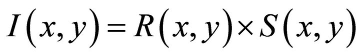 .
.
There are two tracks on the intrinsic image decomposition. One is to extract the reflectance image and the illumination image from a sequence of observed images [7,8]. The other is to extract the reflectance image and the illumination image from a single observed image [9,10]. The typical work for the intrinsic image recovery from a sequence of observed images is from Weiss [8]. He decomposed the intrinsic image from a sequence of images taken under a stationary camera. He assumes that the reflectance is constant and the illumination varies with time. One important natural image statistics is that its derivative filter output is sparse [11,12]. By incorporating the statistics of natural image as a prior, he developed a maximum-likelihood estimation solution to this problem. For the intrinsic image recovery from a single observed image, Tappen, Freeman and Adelson [10] presented an algorithm that incorporates both color and gray-level information to recover shading and reflectance intrinsic images from a single image. They assume that every image derivative is caused either by illumination or by a change in the surface’s reflectance, but not both. In order to propagate local information between different areas, they introduced Generalized Belief Propagation to classify the ambiguous areas.
The work most related to ours is from Finlayson [13]. They devised a method to recover reflectance images directly from a single color image. Under assumptions of Lambertian reflectance, approximately Planckian lighting, and narrowband camera sensors, they introduced an invariant image, which is 1-dimensional greyscale and independent of illuminant color and intensity. As a result, invariant images are free of shadows. The most important step to compute invariant images is to calibrate the angle for an “invariant direction” in a 2-dimensional log-chromaticity space. The invariant images are generated by projecting data, in the log-chromaticity space, along the invariant direction. They showed a fact that the correct projection can be reached by minimizing entropy in the resulting invariant image. In practice, they recovered shadow-free images for the images from unsourced imagery. To minimize the entropy on the projected data seems equivalently to maximize the probabilities within one sensor band. As a result, the color data from one sensor band have minimum variance and then distribute as close as possible after projection. They used histograms to approximate probabilities in every search direction.
Here, we present an intrinsic image decomposition method for a single color image under the above assumptions of Lambertian reflectance, approximately Planckian lighting, and narrowband camera sensors. We showed that the invariant direction could be achieved successfully through the Fisher Linear Discriminant (FLD). We obtain the satisfactory invariant images through FLD. The Fisher Linear Discriminant not only guarantees the within-sensor data as convergent as possible but also treats the between-sensor data as separate as possible. In Section 2, we give a description on invariant direction and invariant image. We discuss the Fisher Linear Discriminant and explain how it can be used to detect the projection direction for invariant images in Section 3. Section 4 shows how to recover the shadow free image from derivative filter outputs. The shadow removal algorithm is proposed in Section 5. In Section 6, experimental results are given to show that the shadow free images could be recovered through the Fisher Linear Discriminant. Finally, we make a conclusion and discuss the future work.
2. Invariant Direction and Invariant Image
Under assumptions of Lambertian reflectance, approximately Planckian lighting, and narrowband camera sensors, a 1-dimensional greyscal invariant image can be generated. The invariant image is independent of illuminant color and intensity. As a result, invariant images are free of shadows. A 2-dimensional log-chromaticity map is first created by calculating the positions of 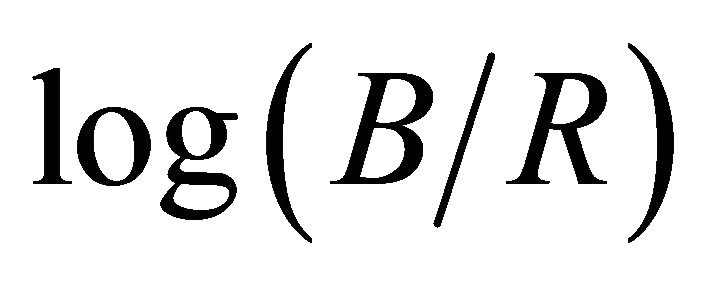 and
and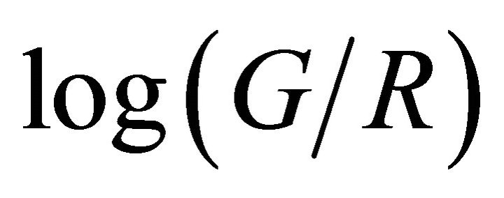 . One amazing property is that points from different illuminant conditions but under the same sensor band tend to form a straight line. Furthermore, those lines from different sensors tend to be parallel. Therefore, if we project those points onto the vertical direction to the lines, we obtain an illumination free image, which is called the invariant image. This is illustrated in Figure 1.
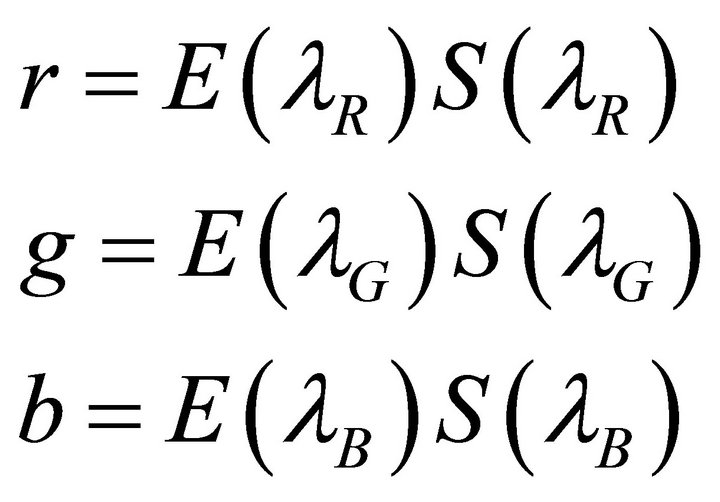
Let us take a look at the theory behind this. The following part of this section gives a brief review on the invariant image theory from Finlayson [13,14]. As we know, camera responses depend on three factors: the light E, the surface S, and the sensor . So we can represent each channel value as integrations over all wavelengths,
 (1)
(1)
If the sensor is narrowband, then we have a Delta function constraint on each channel, as follows
 (2)
(2)
Then the integrations for each channel can be picked at single wavelength as follows
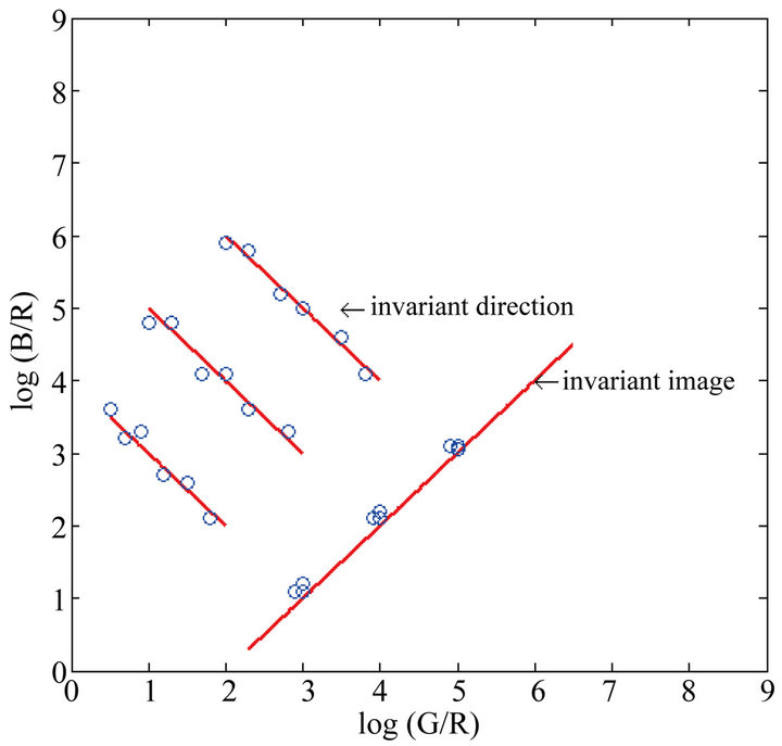
Figure 1. Illustration of the invariant image and the invariant direction.
 (3)
(3)
Most typical illuminants lie on, or close to, the Planckian locus. Under Planck’s law, the light  can be computed as
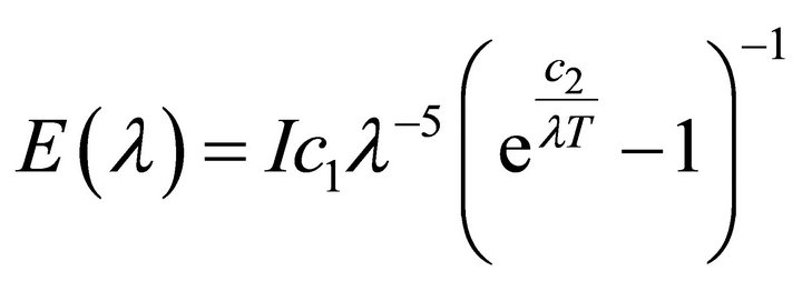 (4)
(4)
where I controls the overall intensity of light, T is the temperature, and  and
and  are constants.
For typical illuminants, we have . Then
  can be approximated as
 (5)
(5)
Furthermore,
 (6)
(6)
 (7)
(7)
On the right hand side of Equation (7), the first element is a constant and independent of sensor. The second element is only dependent on reflectance. For Lambertian surfaces, the reflectance is determined by the surface . The third element is dependent on illumination since temperature
  is inside. Summarizing over three channels, we have
 (8)
(8)
where subscript  denotes dependence on reflectance and k, a, b, and c are constants,
  is the temperature.
By introducing two new parameters  and
and  as follows, we can remove illumination.
 (9)
(9)
We can see that there exists a linear relationship between  and
and , which is free of illumination
 (10)
(10)
That is, if we project log-chromaticity data along the straight line, the projected data are only dependent on surface reflectance.
To compute invariant images requires calibrating the angle for an invariant direction in a log-chromaticity space. Here, we show that the invariant direction can be recovered through the Fisher Linear Discriminant and we got satisfactory results.
3. Invariant Image by Fisher Linear Discriminant
Pattern recognition algorithms that minimize entropy guarantee that the projected data have minimum variance within each class. In our application, the projected data from the same sensor band are required to distribute as closely as possible. The Fisher Linear Discriminant [15] is developed for dimensional reduction and pattern classification. The goal of Fisher Linear Discriminant is to project original data onto low dimensional space such that the between-class distance is as large as possible and the within-class distance is as small as possible. Using the Fisher Linear Discriminant, we not only make the projected data from the same band as convergent as possible, but also separate the projected data from different sensor bands as apart as possible. Therefore, the Fisher linear discriminant is a good choice to choose the invariant direction.
Assume that there are  classes among original data. The data are represented as
  vector
  for
for , where
  is the data dimension and
  is the total number of data. Further, the classes are labeled as
  for
for . We have the following definitions.
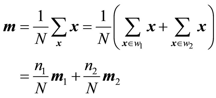
The sample mean for class  is
is
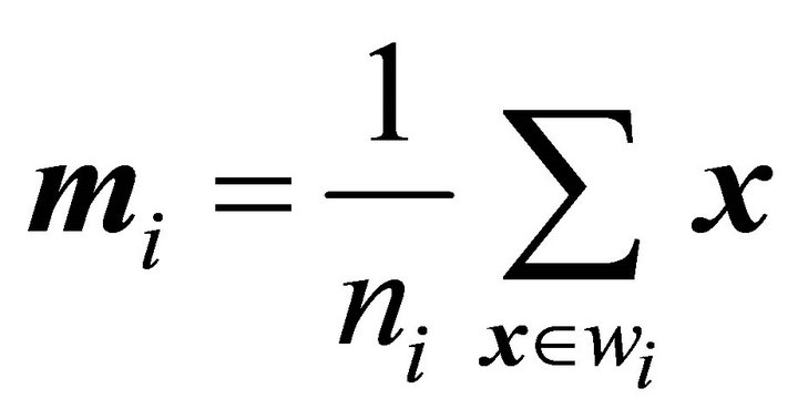 , for
, for  (11)
(11)
where  is the number of data in class
  and
and .
.
The scatter matrix for class  is
is
 , for
, for  (12)
(12)
The total scatter matrix for the whole data is
 , for all samples (13)
where  is the mean for the entire data set.
The between-class scatter matrix is
 (14)
(14)
The within-class scatter matrix is
 (15)
(15)
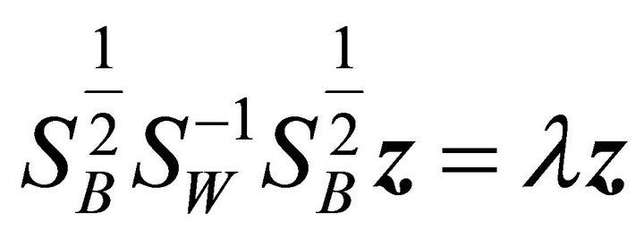
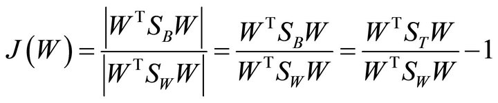
The Fisher Linear Discriminant is to find a  matrix W such that the following optimal criterion
  is maximized.
 (16)
(16)
where  is the determinant of a matrix. The term
  is also called the Rayleigh quotient. The solution to the Fisher Linear Discriminant is the eigenvectors corresponding to the
  largest eigenvalues in the following eigen-problem:
 (17)
(17)
Equivalently,
 (18)
(18)
As a matter of fact, this is a generalized eigen-problem. Since  is symmetric (
 is also symmetric), it can be diagonalized as
 , where U is an orthogonal matrix, consisting of
 ’s orthonormal eigenvectors, and
  is a diagonal matrix with eigenvalues of
  as diagonal elements. Define
 , then
 (19)
(19)
Define a new vector , then
 (20)
(20)
This becomes a regular eigenvalue problem for a symmetric, positive definite matrix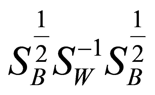 . The original solution can be given as
 .
.
Since we only care for a projection direction for 2-dimensional data, we always compute the unit vector with the same direction as . That is,
 .
.
Since
 (21)
(21)
remember that
 (22)
(22)
Similarly,
 (23)
(23)
In addition,
 (24)
(24)
We obtain
 (25)
(25)
In our case, we want to find a projection line in 2-dimensional space. So  equals
 (26)
(26)
3.1. Special Cases for Fisher Linear Discriminant
In practice, it always happens that there are at most two classes in the 2-dimensional chromaticity space. Then Fisher linear discriminant is considered as follows.
Case 1. There are only two classes.
In this case, the total mean is
 (27)
(27)
Substituting this in
 (28)
(28)
We obtain
 (29)
(29)
Similarly,
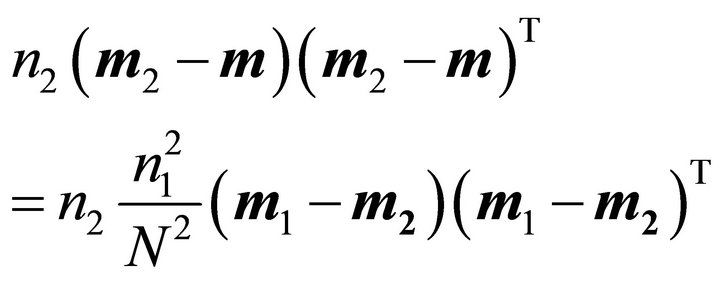 (30)
(30)
Then the between-class scatter matrix becomes
 (31)
(31)
where  means “equals up to scale”.
Since we only care about the direction of projection, the scale can be ignored. From Equations (17) and (18), we obtain the projection  as
as
 (32)
(32)
where  is just a scalar.
Case 2. There is only one class.
The 2-dimensional data distribute along parallel straight lines. We hope that the invariant direction is the direction with the minimum-variance for the withinsensor data. That is, the projected data from the same sensor distribute as close as possible. If there is only one class in the 2-dimensional chromaticity space, the eigenvector corresponding to the smaller eigen-value for the 2-dimensional chromaticity data matrix will be the invariant projection direction. This is different from principal component analysis for dimensional reduction, where the eigenvectors corresponding to the largest eigenvalues are chosen for projection.
3.2. K-Means Method for Clustering
Before applying the Fisher linear discriminant, we need to classify the original data into different groups. That is, we need to solve which class each datum belongs to and assign each datum accordingly. This is accomplished through the K-means algorithm [16]. Given the number of clusters, the K-means method partitions the data iteratively until the sum of square distances for all data to its class center (total intra-cluster variance) is made to be minimum.
It is possible that other algorithms such as Gaussian mixture models may give a better result. However, in practice, the K-means algorithm works well here. Figures 2 and 3 illustrate the Fisher linear discriminant for one class and three classes, where clustering is implemented through the K-means method. We can see that we have obtained satisfactory invariant images through data projection on the invariant direction chosen by Fisher linear discriminant method. In practice, we found that accurate invariant images are not necessary to remove illumination. However, the accurate shadow edge detection is very important for shadow removal.
4. Recovery of Shadow Free Images
It is suggested by Weiss [8], that we can reintegrate the derivative filter outputs to generate shadow free images and further recover intrinsic images. We compute the derivative filter outputs for R, G, and B color channels respectively and then set the derivative values in shadow edge positions to zeros. Finally, we reintegrate the derivative filter outputs back to recover the shadow free images Here, we simply consider derivative filters as the horizontal derivative filter and the vertical derivative filter. The horizontal derivative filter is defined as
 and the vertical derivative filter is
 .
.
After we have individual reflectance derivative map, where derivative values in shadow edge positions are set to zeros, following Weiss [8], we can recover the reflectance image through the following deconvolution.
 (33)
(33)
where  is the filter operation and
  is the reverse filter to f. r are the derivatives and
  are the estimated reflectance image. Further, g satisfies the following constraint.
 (34)
(34)
In practice, this can be realized through the Fourier transform.
5. The Shadow Removal Algorithm
In summary, our algorithm to remove shadows for a single color image consists of the following steps:
1) Compute the 2-dimensional log-chromaticity maps for original color images;
2) Cluster data in 2-dimensional log-chromaticity space using K-means algorithm;
3) Compute the invariant direction (projection line) using Fisher Linear Discriminant;
4) Generate the invariant images by projecting 2-dimensional data along invariant direction;
5) Compute the edge maps for graylevel image (each channel of R, G, B) of the original images and graylevel invariant image using Canny edge detectors;
6) Extract those edges in original edge maps but not in invariant image edge map as shadow edges;
7) Compute the derivative filter outputs for R, G, and B color channels;
8) Set the derivative values in shadow edge positions to zeros;
9) Reintegrate the derivative filter outputs back to recover shadow free images.
6. Experimental Results
In test, we conducted the shadow removal algorithm on four real pictures, where the data are either collected by us or collected online. In addition, the data are not taken under the same illumination. The outcomes are displayed in Figures 4-7. The invariant images are produced through FLD as shown in (b) of Figures 4-7. The Canny edge detector is applied to extract edges in invariant image and gray-level images for each channel R, G, B of the original color image. In comparison with invariant image and gray-level images for each channel R, G, B, we can see that the shadow edges are basically extracted correctly. The edge detection is shown in (c) of Figures 4-7. Then derivatives in edge positions are set to zero values and further reintegrated back. The shadows in the recovered images are either considerably attenuated or effectively removed (refer to in (d) of Figures 4-7). We also notice that some artifacts exist in the recovered images. This results from inaccurate shadow edge detection.
7. Conclusion
In this paper, we give an effective approach to recover shadow free images from a single color image, which is from unknown source. This is an improvement way that used by Finlayson [13,14]. In our experiments, we feel that accurate invariant direction is not necessary. In reality, the data in 2-dimensional log-chromaticity space from different sensors are not right parallel. However, after projection through the Fisher Linear Discriminant, we can still obtain satisfactorily invariant images. In the future work, we will work on automatic selection of number of cluster components for the K-means method. This may be achieved through cross-validation on different number of cluster components. The other clustering method instead of the K-means method may be explored in our future experiments.