Convergence and Error of Some Numerical Methods for Solving a Convection-Diffusion Problem ()
1. Introduction
In this paper we present an eoretical study of the smoothing, convergence and error reduction properties of the multigrid method for a time dependent convection diffusion equation. This is an equation that arises in the mathematical modeling of many physical phenomena, which makes the efficient numerical solution very important.
The equation studied here models the transport of molecules through the layers of the skin, until it reacheas the blood stream. The parameters used for the diffusion coefficients are smaller by several order than those of the convection, thus the equation is a convection dominated one.
The discretization of the differential equation is realized by two different methods: the finite difference method [1] with Euler backward discretization and the Galerkin finite element method [2,3].
The system obtained after the discretization process is solved using the multigrid method. This method was first introduced by Fedorenko [4,5]. The first practical results and efficiency of the method were given by Brandt [6,7].
The theory of multigrid convergence is well established for the Poisson equation [8-10]. In more recent articles the convergence has been studied for the convectiondiffusion equation [11,12].
The novelty in this paper is that we study the smoothing factor, asimptotic convergence factor and the error reduction factor of the multigrid method for a time dependent convection-diffusion equation, on a domain comprising three layers with different physical properties. The analyse is performed using the local Fourier techniques [9,13] which represents a good tool for constructing efficient multigrid methods for a given differential equation.
We also determined the error obtained for a given solution of the model problem, using the multigrid method on different number of grid levels, for both discretization methods mentioned above.
2. Mathematical Model
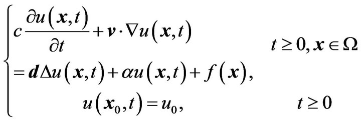
 represents the concentration of the substance transported through the blood stream,
  is the vector of convection coefficients and
  is the vector of diffusion coefficients.
The substance which is transported through the skin is applied at the surface on an area with a radius of a few centimeters. The depth to which the active substance is transported by the diffusion and convection process is of the order of nanometers, thus much smaller than the radius of the surface where it is appplied. As a consequence, the problem can be reduced to the unidimensional case. From this point on, the variable  will represent the depth where the concentration is to be calculated, and the vectors
  and
and  are the coefficients in different layers of the skin.
The concentration of the substance applied on the skin is known, and the amount of it is sufficiently large to be constant at any moment of time :
:
 (1)
(1)
this being the initial condition of the problem.
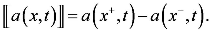
On the frontiers between the skin layers the law of flux conservation gives:
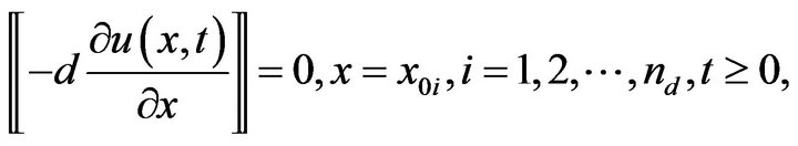 (2)
(2)
 is the number of layers where the diffusion takes place and:
After the discretization process, the system obtained from the Equation (1) has the form:
 (3)
(3)
 .
.
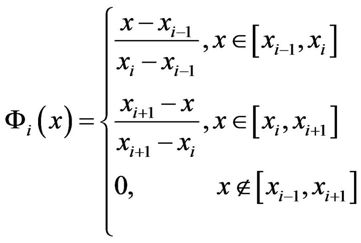
If the finite elements method [14] is used, the weak formulation of Equation (1) gives:
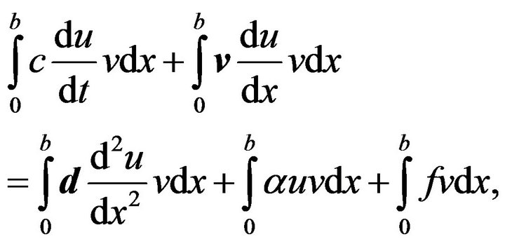
 is a function that has a derivative of order 1 and is square-integrable on
 . The functions
  and
and  are approximated using the continuous functions
 ,
,  being the number of interior points of the grid on level
 , through the relations:
 . Replacing the functions
 and
and  with these approximates and using the standard integration-by-parts formula the equation becomes:
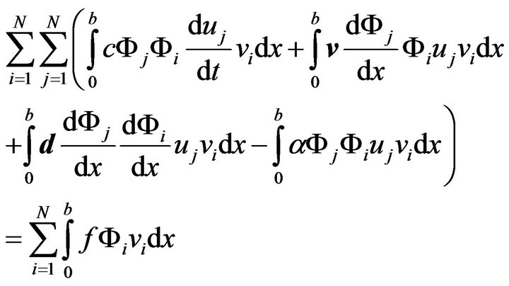
or:
 (4)
(4)
Computing the integrals from (4) for
the coefficients in the system (3) are:
 (5)
(5)
For the finite differences method using the explicit backward Euler scheme:
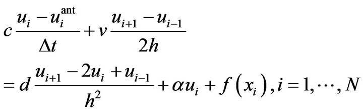
the coefficients for the system (3) will be:
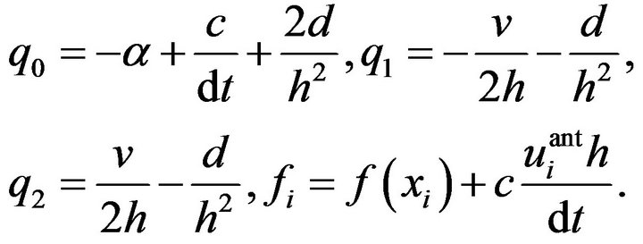 (6)
(6)
In the nodes that are on the frontiers between different layers of the skin , the law of flux conservation (2) becomes:

In these points the system (3) has the coefficients:
 (7)
(7)
3. The Components of the Multigrid Method
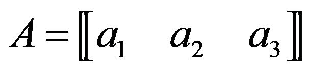
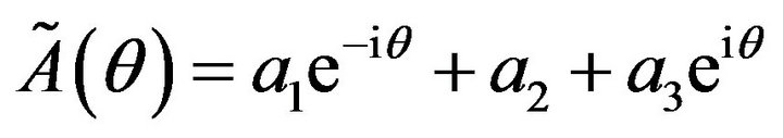
For the components of the multigrid method we give in the following the matrices associated to their operators, needed for the local Fourier analysis of the convergence. The essential property used by this method is the fact that the discretiztion of the problem leads to a system that has the eigenvectors equals to the Fourier modes and when the multigrid components have a block structure when computed in the Fourier basis, the analysis of the multigrid method is reduced to the one of diagonal blocks of small size.
3.1. The Matrix of an Operator
If  is an operator that can be described by a difference stencil:
meaning that:

then the functions 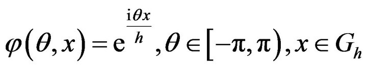 are the eigen functions of
 :
:
 (8)
(8)
and:
are the eigenvalues of .
.
As , it is sufficient to take
 .
.
If , the set of low frequencies, then:
 is the set of high frequencies.
Using the above notations, for an arbitrary function
 , the operator
  applied to
  gives:

and  represents the matrix associated with the operator
 .
.
3.2. The Operator of the Discretized System
 from system (3) applied to a function
  will give:
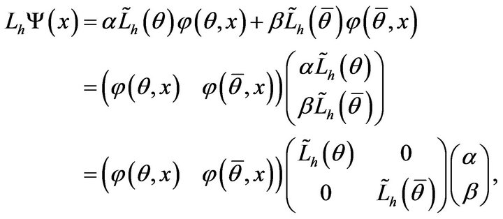
where .
.
Thus the matrix of 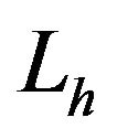 is:
is:
 (9)
(9)
3.3. Preand PostSmoother
The Gauss-Seidel red-black method is used before and after the coarse grid correction, and reduces well the high frequency components of the error. The smoothing operator has two components of Jacobi type:

In the relations above:
 (10)
(10)
As:

the matrix of the smoother will be:
 (11)
(11)
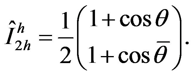
3.4. Restriction of the Defect
Full-weighting restriction is used as a fine to coarse grid transfer operator :
As
 (12)
(12)
the restriction operator applied to the function 
 will give:
 (13)
(13)
with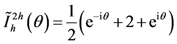 .
.
Thus the restriction operator has the matrix:
 (14)
(14)
3.5. Solution on the Coarse Grid
In the two-grid method, the exact solution on the coarse grid is required. After the restriction of the defect, the function on the grid  has the form
 (12,13). Thus:
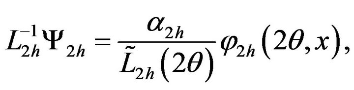
wherefrom the matrix of the operator is:
 (15)
(15)
3.6. Prolongation
The coarse to fine interpolation operator used is the bilinear interpolation:

From this relation it follows that:

and the matrix of the prolongation operator is:
 (16)
(16)
3.7. Two-Grid Operator
The multigrid method [8,15] is a combination between a relaxation method (that reduces very well the high frequency components of the error, but is slowly convergent because of the low frequency components) and the coarse grid correction (which has complementary properties to the smoother).
The matrices from (9), (11), (14), (15) and (16) are used to create the two-grid operator for the multigrid method:
 (17)
(17)
where:
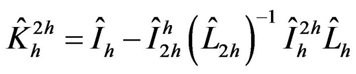 (18)
(18)
is the matrix of the coarse grid correction operator.
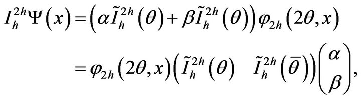
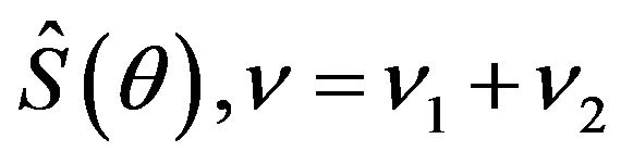
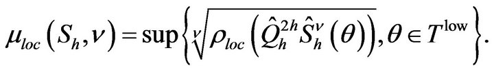
It has been proven [9] that it is sufficient to derive the convergence properties for the two-grid method and the multigrid method will have similar properties. As a consequence, the following factors are defined for the two-grid operator.
Asimptotic convergence factor
 (19)
(19)
Error reduction factor
 (20)
(20)
Here:  denotes the spectral norm associated with the Euclidian vector norm in
 , and
, and
 (21)
(21)
Smoothing factor
 (22)
(22)
where  is the spectral radius of the matrix
 .
.
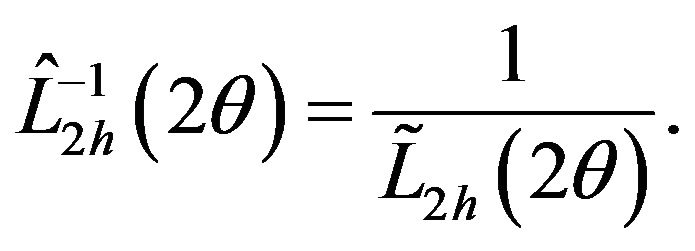
 , introduced in [9], is an "ideal" coarse grid operator that anihilates the low frequency error components and leaves the high frequency components unchanged:

and:
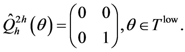
Since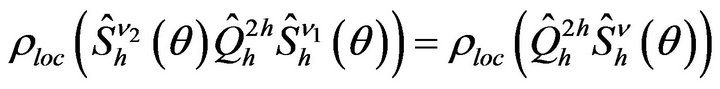 ,
,
 (23)
(23)
4. Local Fourier Analysis Results for the Studied Problem
4.1. Smoothing Factor
If  then the matrix (11) of the smoother after
 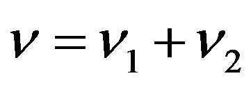 steps is:

and has the eigenvalues:
 and
and  being given in (10),

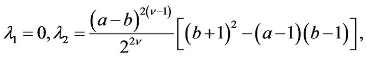
For , the eigen value
  attains its maximum absolute value:
 (24)
(24)
for . The smoothing factor for the problem (1) is:
 (25)
(25)
Here,  are the coefficients given in (5)-(7).
For a = 10−4, ct = 1, d1 = 1 × 10⁻¹², d2 = 1 × 10⁻¹⁰, d3 = 3 × 10⁻¹⁰, v1 = 1 × 10⁻⁹, v2 = 1 × 10⁻⁶, v3 = 1 × 10⁻⁶, the smoothing factors for the Gauss-Seidel relaxation method are presented in Table 1.
The data from Table 1 show that:

Table 1. The smoothig factor as a function of  and
and .
.
the Gauss-Seidel red-black relaxation method is a very good smoother for this problem as the smoothing factors in the cases presented here are ;
;
both the discretization methods lead to good smoothing factors. The finite element method seems slightly more appropriate when the number of grids used in the multigrid method is bigger;
the number of relaxation steps before and after the coarse grid correction should not be too big as the smoothing factor increases with .
.
4.2. Asimptotic Convergence Factor and Error Reduction Factor
For the multigrid method having the components described in (9-16), the matrix of the two-grid operator for the problem (1) is:
 (26)
(26)
For  the corresponding asimptotic convergence factor and error reduction factor have been computed from the matrix (26) and are given in Table 2 for different numbers of preand postsmoothing steps.
The data from Table 2 show that the multigrid method is very rapidly convergent: if at least one smoothing step is performed before and after the coarse grid correction, then the error is reduced by at least a  factor per multigrid cycle.
5. Numerical Results
The problem (1) has been solved on a domain containing tree layers with different diffusion and convection coefficients ([16,17]).
The error was computed for the exact solution
The time step in the discretization process has been . Figure 1, Figure 2 and the Table 3 represent the error after eight multigrid cycles, with two smoothing steps before and two after the coarse grid correction.

Table 2. Asimptotic convergence factor and error reduction factor .
.
 (a)
(a) (b)
(b)
Figure 1. The multigrid error at ad = 100 nm in the skin for v1 = 1.0 × 10⁻¹⁰, v2 = 1.0 × 10⁻⁷, v3 = 1.0 × 10⁻⁷, d1 = 1 × 10⁻¹², d2 = 1 × 10⁻¹⁰, d3 = 3 × 10⁻¹⁰; c = 104; a = 0.
 (a)
(a)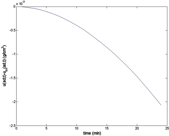 (b)
(b)
Figure 2. The multigrid error at ad = 100 nm in the skin for v1 = 1.0 × 10⁻⁹, v2 = 1.0 × 10⁻⁶, v3 = 1.0 × 10⁻⁶, d1 = 1 × 10⁻¹², d2 = 1 × 10⁻¹⁰, d3 = 3 × 10⁻¹⁰; c = 103; a = 0.
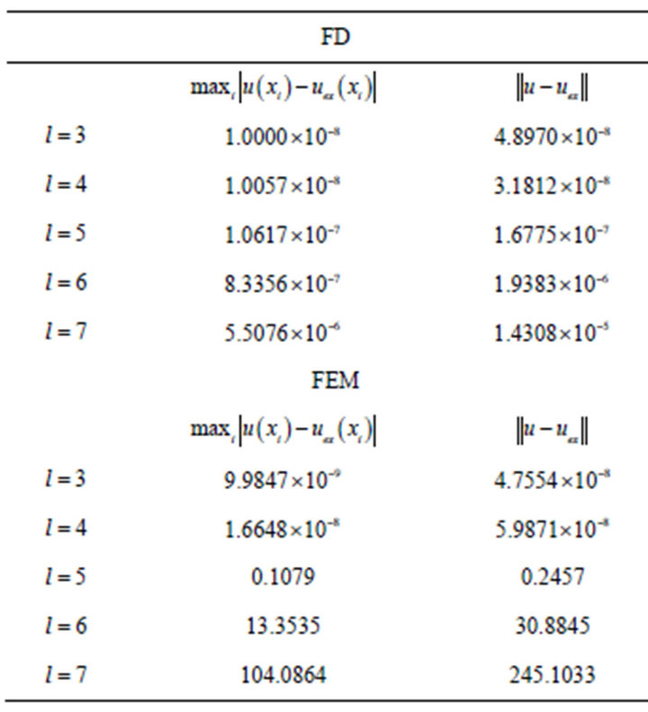
Table 3. Multigrid error for FD and FEM.
Table 3 shows the maximum absolute value of the error and the norm of the error vector corresponding to Figures 1(a) and (b), for the finite differences discretization method (FD) and finite element method (FEM).