A New Algorithm for Computing the Determinant and the Inverse of a Pentadiagonal Toeplitz Matrix ()
1. Introduction
Pentadiagonal Toeplitz matrix linear systems often occur in several fields such as numerical solution of differential equations, interpolation problems, boundary value problems [1-5], etc. In these areas, the determinants and the inversions of pentadiagonal Toeplitz matrices are considered. In recent years they have become one of the most important and active research field of applied mathematics and computational mathematics increasingly.
In [2], E. Kilic, M. Ei-Mikkawy presented a fast and reliable algorithm with the cost of  for evaluating special nth-order pentadiagonal Toeplitz determinants. In [1], X.G. Lv, T.Z. Huang, J. Le presented an algorithm with the cost of
  for calculating the determinant of a pentadiagonal Toeplitz matrix and an algorithm for calculating the inverse of a pentadiagonal Toeplitz matrix.
In this paper, we present new algorithms for computing the determinant and the inverse of an n-by-n pentadiagonal Toeplitz matrix. The complexity of the algorithms are  and
and  respectively.
This paper is organized as follows: in Section 2, we present some useful notations and lemmas. In Section 3, we are going to derive new two algorithms. Finally, we give an numerical examples to show the performance of our algorithms in Section 4.
2. Notations and Preliminaries
Definition 2.1 Let  be an
be an  matrix.
is called persymmetric if it symmetric about its northeast-southwest diagonal, i.e.,  for all
  and
and .
.
Definition 2.2 Form as
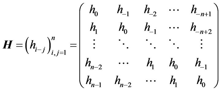
is called Toeplitz matrix.
Toeplitz matrices are all persymmetric matrices.
Lemma 2.1 [6] Let  be an
be an  matrix. Then
(1)  is persymmetric matrix if and only if
  ;
;
(2) If  is nonsingular Toeplitz matrix,
  is also a Toeplitz matrix, where
  is the
  exchange matrix, i.e.,
  ,
,  is the ith column of identity matrix
  of order
 .
.
Without loss of generality, we suppose  in the paper. By computing simply, we have the following conclusion:
Lemma 2.2 Let  be an
be an  Toeplitz matrix
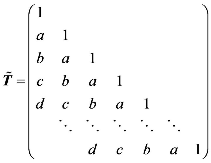 (2.1)
(2.1)
Then the inverse of  is an
is an  Toeplitz matrix, and
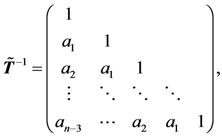
where

and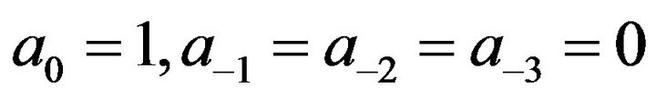 .
.
Lemma 2.3 Let 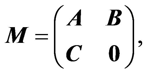 where
where  and
and
 are matrices of size
 respectively.
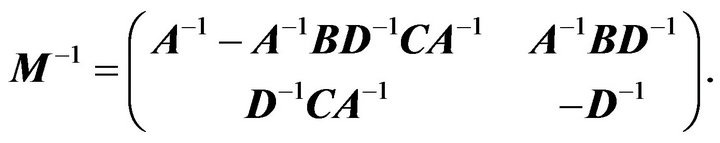
  is nonsingular. Then
  is nonsingular if and only if
 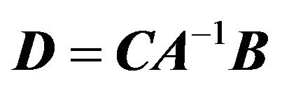 is nonsingular, and
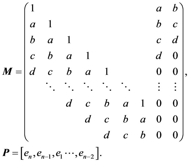
In the current paper, we consider the  pentadiagonal Toeplitz matrix of the form
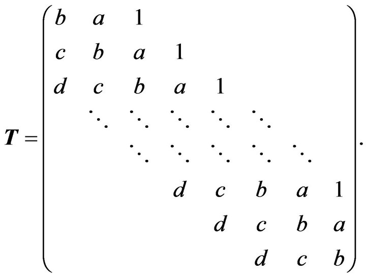 (2.2)
(2.2)
3. Main Results
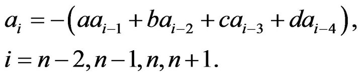
Decompose the pentadiagonal Toeplitz matrix  (2.2) as the following:
where
Partition M into 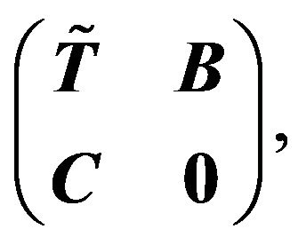 where
where  is matrix (2.1),
 is zero matrix of size
 ,
,
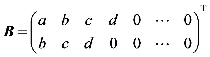 of size
  and
and
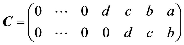 of size
 .
.
Thus

where
Denote
Thus

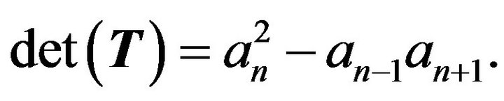
It is noticed that
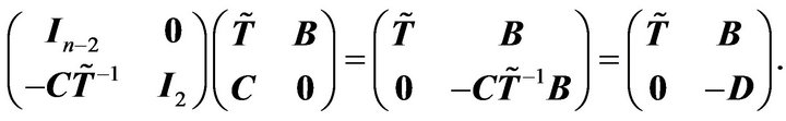
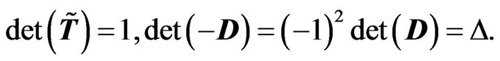
We have
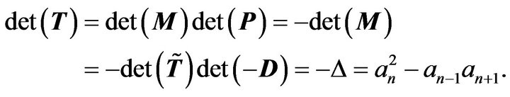
According to the Lemma 2.3 and deduction above, we have the following results:
Theorem 3.1 Let  be the pentadiagonal Toeplitz matrix as (2.2), then (1)
  is nonsingular if and only if
 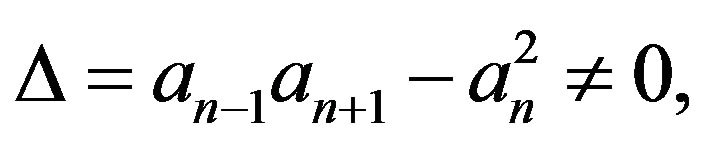 and
and
(2) 
When  , we have that
  is nonsingular, and
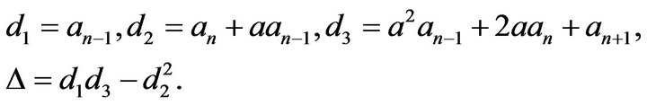
where

and 
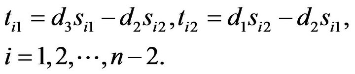
Denote  and
and
 We have

i.e.,
 (3.2)
(3.2)

i.e.,
 (3.4)
(3.4)
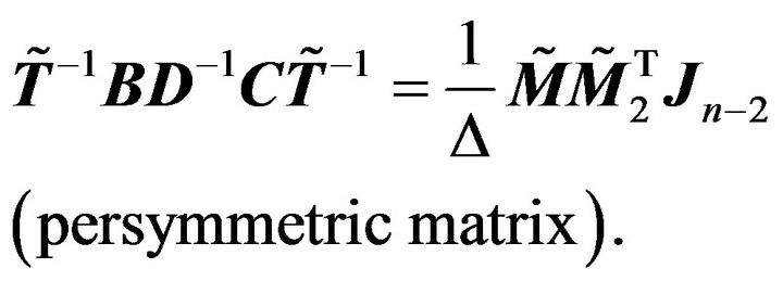
From the Lemma 2.1 and 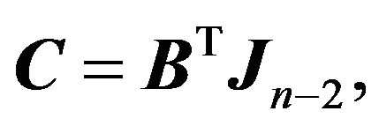 we have
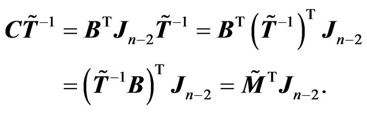
Thus
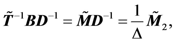

Denote
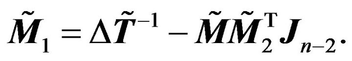 (3.5)
(3.5)
Then 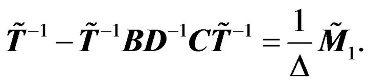
According to the deduction above, we can obtain Theorem 3.2:
Theorem 3.2 Let the pentadiagonal Toeplitz matrix  as (2.2) be nonsingular. Then
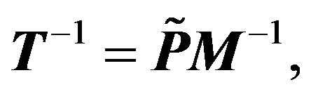
where

 as above.
Combining with Theorem 3.1 and Theorem 3.2, we obtain the following algorithm:
Algorithm 3.1 (Computing )
)
(1) Input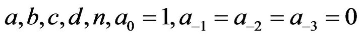 ;
;
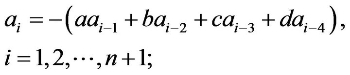
(2) Compute
(3) Compute 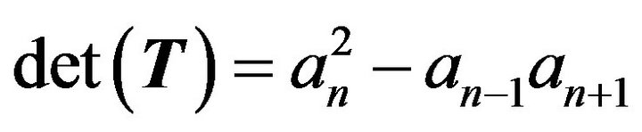 .
.
Algorithm 3.2 (Computing )
)
(1) Using (3.1), calculate ;
;
(2) Using (3.2), calculate ;
;
(3) Using (3.4), calculate ;
;
(4) Using (3.3) and (3.5), calculate ;
;
(5) Calculate ;
;
(6) Calculate .
.
Let us now have a look at the number of multiplications and divisions executed by Algorithm 3.1 and 3.2. For Algorithm 3.1, in Step 2, it takes about  operations. Step 3 amounts to 2 operations. On the whole, we need about
  operations to compute
 . Algorithm 3.1 is better than E. Killic’s algorithm [2] with the cost of
  and X.G. Lv’s algorithm [1] with the cost of
 . For Algorithm 3.2, in Step 1, it takes 4 operations. Step 2 amounts to
  operations. Step 3 amounts to
  operations. The cost of step 4 is about
 , we make use of the persymmetric matrix. Therefore, we need about
  operations computing
 . Our algorithm is better than X.G. Lv’s algorithm [1] with the cost of
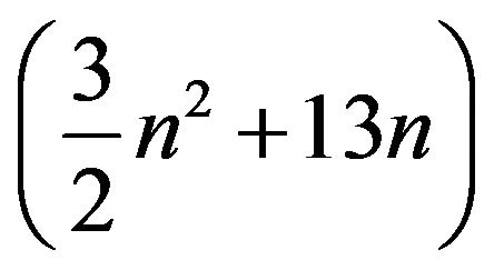 .
.
4. An Example
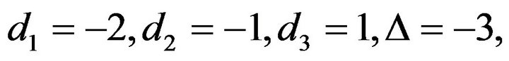
Consider the pentadiagonal Toeplitz matrix as
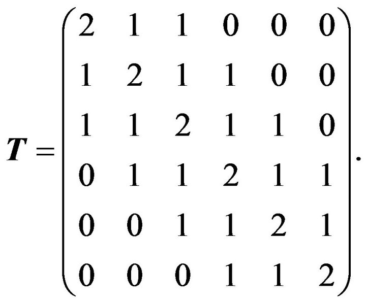
By Algorithm 3.1, we have
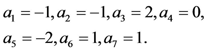
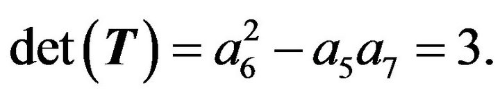
So
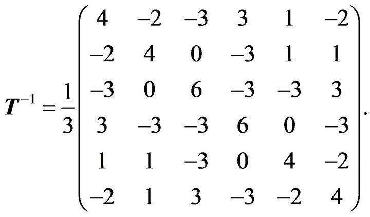
Using Algorithm 3.2, we obtain
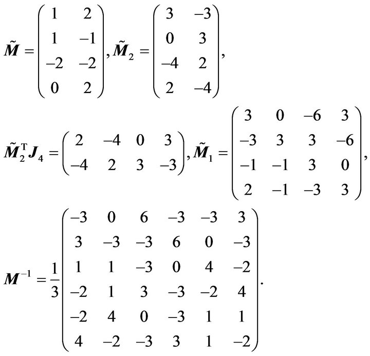
So
NOTES