A New Approach to the Optimization of the CVRP through Genetic Algorithms ()
1. Introduction
The complexity of distribution problems is the reason for the lack of solution techniques able to provide optimal solutions to real cases in a reasonable time [1]. But firms have to make decisions on transportation matters, sometimes in the short run. The economic importance of moving people and goods makes it necessary the development of strategies to generate quick competitive solutions [2,3]. In the literature, these problems are generically known as the Vehicle Routing Problem (VRP) [4], which is NP-Complete combinatorial optimization problem. Its scholarly and practical interest stems from the aforementioned lack of quick solution methods [5]. The main goal of this paper is to introduce a new algorithm, robust, flexible and fast enough to solve different instances of this problem.
The rest of the paper is organized as follows. Firstly, we present some characterizations of the VRP as well as of the original version of the CVRP (Capacitated Vehicle Routing Problem). Then, we introduce an alternative version of the latter and a methodology for its solution. We present later the result of the experiments with this method. Finally we discuss possible further work on the subject.
2. Definition of CVRP
In rough terms, the statement of the VRP is: given classes of clients and of storage sites (both scattered over a geographical region) and a fleet of vehicles, determine the minimal cost routes starting and ending in storage sites delivering the goods to the clients. The features of clients, storage sites and vehicles, as well as the operational constraints over routes determine the different variants of the problem. Each client is associated to a demand that has to be covered by a vehicle. This demand is usually understood as an amount of a good that occupies some volume of the vehicle. In crowded area a single vehicle may not be able to satisfy the demands of all the clients living there. The capacity of the vehicle imposes then a bound on the number of clients that it might satisfy at the same time [6,7]. This kind of constraints defines the CVRP (Capacitated Vehicle Routing Problem). The capacity of the vehicle might be in terms of weight or volume. When more than a single kind of products is transported the vehicles could be compartmented carrying each type of parcel in a different subdivision. A distinction can be made between the problems of homogeneous fleets, in which the attributes (capacity, cost, etc.) are the same for all the vehicles, and heterogeneous fleet problems. The latter case raises the possibility of incompatibilities between the capacities of the vehicles and the demands of the clients. If then, each client might be visited only by some of the vehicles. It could also happen that the goods to be transported might not be available in a single storage site and must be collected from several sites. All these depots have to be visited before delivering the goods to the client. While normally each client should be visited once, it could be necessary to satisfy his demand at different moments and by different vehicles. Some clients could have some hourly restrictions for the reception of parcels, which are expressed as time windows [8,9]. In such case the problem is known as VRPTW (Vehicle Routing Problem with Time Windows). The vehicles, as well as the products, are usually parked at the storage sites. It is also usually required that the vehicle starts and ends trips from the same storage site, but this restriction can be lifted in some cases. The number of available vehicles could be given or be decision variable [10]. The objective is frequently the minimization of the distances as well as the number of vehicles used while satisfying the demands of the clients [11,12]. Recent studies have allowed the possibility of vehicles traversing different routes [13]. Different presentations of such problems can be found in the literature [14-17], as well as different approaches to solving them [18-23].
In this work we focus on the CVRP. Consider version (1) of the problem. Let  be the class of client nodes, endowed with a linear order <,
  the set of storage nodes while
 .
.  the cost (distance) of going from nodes i to j for any pair
 .
.  is a binary variable, which is 1 if a vehicle goes from i to j without intermediate stops. Otherwise
 .
.  is the maximum capacity of a vehicle and
  the amount demanded at a node
 . Let
. Let  be the class of nodes in a path that starts and ends at node
 . Then, the problem is:
 (1)
(1)
s.t.:
1) 2) and
  such that
In words: minimize the total distance traversed by all vehicles, satisfying the demands on every route for a partition of client nodes in clusters, each one covered by a single vehicle. Notice that constraint 2) makes the problem more complex than a linear programming one.
Version (2) is as follows: let  for some allocation of routes,
  the sum of distances over route m,
  is a binary variable that is 1 if route m is used and 0 otherwise and
  also a binary variable (1 if
  belongs to route m and 0 otherwise). Then, the problem is:
 (2)
(2)
s.t.:
3) and for each i,  That is (2) is analogous to (1) under constraint 1) with constraint 2) already satisfied.
3. Methodology
An algorithm solving (2) proceeds in two stages. The first one generates feasible clusters, classifying and ordering them. The second stage solves the minimization problem by means of a Genetic Algorithm [24].
3.1. First Stage
The algorithm generates the clusters that will be elements of .We take each
  and consider all the clusters
  such that
 . The inductive construction starts with i = 1 (the lowest in the < order) building all the clusters of client nodes that include 1, satisfying condition 1). Then, if all possible clusters up to i = k have been obtained, consider i = k +1 (where, of course, k < k + 1). All routes starting and ending in a node of
  that go through client nodes in
 , including node k + 1, satisfying condition 1), are constructed.
For each  its class of clusters, denoted Si, is endowed with a weak order Ði (reflexive, antisymmetric and transitive, i.e. allowing ties) according to the number of clients in each cluster. Among clusters covering the same number of client nodes, say
  and
and , if k < l then
  Ði
Ði . The highest rank in Ði corresponds to routes covering i as well as the largest possible number of other client nodes in the upper level of order <. As an example, consider the case of 10 client nodes demanding 50 units and a vehicle capacity of 100 units. Table 1 shows the distances among nodes, being 0 the storage site from which departs the vehicle. Table 2 shows the result of the first stage of the procedure. Notice that, since the capacity of the vehicle is 100 and each client node demands 50, a route that clusters some clients together can only consist of two of them. So, for instance the group corresponding to node 9 includes only two possible clusters, {9} and {9,10}, because all other nodes have already been assigned to other clusters. Cluster {9,10} is of a higher order than {9} because it includes two clients instead of just one node.
3.2. Second Stage
At this point a Genetic Algorithm [24] is applied, designed for its use in this problem. An individual is codified in a chromosome constructed in such way as to satisfy conditions 2) and 3) and therefore are feasible under problem (2). The coding operates on a lexicographic basis. Each  is given a number, starting with i = 1, and following the process according to order <. So, take all the clusters ordered according to Ð1. This order can be represented by the linear numerical order
 . So, if the k-th cluster in the ordering is chosen, the corresponding gene in the chromosome is k. For i = j, the

Table 1. Distances—Case: 10 nodes / Demand per node: 50 units / Vehicle capacity: 100 units.

Table 2. Clusters—Case: 10 nodes / Demand per node: 50 units / Vehicle capacity: 100 units.
order Ðj is applied to a subset of  obtained by eliminating (“filtered out”) all the clusters that include nodes already present in clusters corresponding to genes i = 1,···, j – 1. The new ordering is denoted
 . Then the j-th gene in the chromosome is the rank in
  of the cluster that is chosen. If for a given i the domain obtained is Æ (because all possible nodes belong to clusters corresponding to genes 1 to i – 1), any number between 1 and
  can be assigned to the i-th gene. In this way, a chromosome is defined, each corresponding to a feasible solution to problem (2). The Genetic Algorithm seeks to find the optimal one.
We can see some examples of how chromosomes encode clusters in Table 3, (3-3-2-1-4-2-3-2-1-1) and Table 4 (5-2-1-5-1-4-2-2-1-1): all routes start and end at node 0 and go through two client nodes; in gray we see the filtered out clusters and in red the selection. Consider for instance the second gene in Table 3: it has to discard (written in gray) all routes that go through node 3, since it has already been assigned to the first gene. Number 3 assigned to this gene indicate that the route selected is the third in the list of non-filtered routes. On the other hand, a number assigned to a gene with a row with all routes filtered out does not have any effect. The initial population consists of individuals whose chromosomes are constituted by genes selected at random. Once established a chromosome, it is decoded and evaluated. This evaluation is performed according to problem (2). For the computation of each cluster we use Lin-Kerninghan’s algorithm that yields the minimal distance among its nodes. The following operators have been chosen in the light of some previous evaluations. The cross-over operator is the two-point one (Table 5, Parent 1: 3-3- 2-_-_-_-_-2-1-1, Parent 2: _-_-_-5-1-4-2-_-_-_, Offspring: 3-3-2-5-1-4-2-2-1-1) and the mutation operator alters gene values at 10% of the chromosome (Mutation (Table 6, Offspring*: 3-3-2-5-1-2-2-2-1-1)). Finally, the selection is by ranking.
The Genetic Algorithm runs until the solution gets stabilized. These tests were implemented with a C++ program running on a 3.00 GHZ CPU with a 2.00 GB RAM. The parameters of the experiments were as follows. The size of the population: 100; the cross-over probability: 0.70 and the probability of mutation: 0.01.
Before running the algorithm over problems in the literature we experimented over this example. Figure 1 shows the nodes and their proportional distances in a two-dimensional framework. Figures 2 to 7 show the

Table 3. Example of a chromosome ( 3-3-2-1-4-2-3-2-1-1) that will act as parent 1 in the cross-over of Table 5.

Table 4. Example of a chromosome ( 5-2-1-5-1-4-2-2-1-1) that will act as parent 2 in the cross-over of Table 5.

Table 5. Cross-over (offspring: 3-3-2-5-1-4-2-2-1-1).

Table 6. Mutation (offspring*: 3-3-2-5-1-4-2-2-1-1).
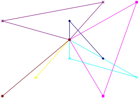
Figure 2. Generation 10, distance: 205.61.

Figure 3. Generation 20, distance: 205.56.

Figure 4. Generation 45, distance: 201.65.
routes generated in several generations and the minimal total distance covered by the selected routes.

Figure 5. Generation 75, distance: 201.40.

Figure 6. Generation 100, distance: 169.76.

Figure 7. Generation 150, distance: 153.06.
4. Experiments and Results
Van Breedam [25] presents a large number of instances of features and values. He suggested also a reduced set of representative cases to be solved by different heuristics. Some of them involve 100 nodes with a total demand of 1000 units. We follow here this convention and use the author’s nomenclature for the cases with the same capacity of vehicles. The problems tested range from Bre-1 to Bre-15. From Bre-1 to Bre-6 only the capacity of vehicles is restricted. The demand on each client node is 10 units, while the vehicle capacity is 100 units in Bre-1 and Bre-2, 50 units in Bre-3 and Bre-4, while it is of 200

Table 7. Results for the problems of Van Breedam [25,26].
units in Bre-5 and Bre-6. Problems Bre-7 and Bre-8 have not been considered because they involve both deliveries and pickups. In most of these problems a single type of good is assumed. Exceptions are problems Bre-9 to Bre-11, in which demands are heterogeneous. Finally Bre-12 to Bre-15 are problems involving time windows, and therefore are not included in our experiments. Table 7 presents the results of our tests. The best known solution, drawn from [25,26], is presented as well as information on the solutions under our procedure (best solution, average evaluation, success, mean solution, average running times and percentage of difference with the best known solution). With respect to the processing time, some instances took only minutes while others required hours, although in average the best solutions took not much longer than an hour to be found.
5. Conclusion
We presented a new algorithm for the CVRP (Capacitated Vehicle Routing Problem), distinguishing between the standard and its alternative formulation. The details of the procedure were described and the comparison with results in the literature has been presented. While the outcomes are similar to them, their running times are not. In experiments not discussed here we noticed that problems that exceed 100 nodes the processing time is much longer, due to the demands of the first stage of the algorithm. We plan to add further search filters at the optimization stage as well as to try with other meta-heuristics to run on the alternative model.
6. Acknowledgements
This work has been supported by several funding sources. The authors are in particular thankful to the National Research Council of Argentina (CONICET) as well as to the Universidad Nacional del Sur project PGI 24/J056.