Research on Credit Risk Assessment of Small and Medium-Sized Enterprises in Commercial Banks

Yacui Gao, Lidan Zhang

College of Management, Xi’an University of Science and Technology, Xi’an, China.

DOI: 10.4236/oalib.1105022                

Abstract

By using the data of 2014 and 2015 about the 90 small and medium-sized en-terprises credit default and normal samples from a joint-stock commercial bank, this paper builds the credit risk assessment evaluation index system to the small and medium-sized enterprise of commercial bank. Based on the logit model, we make a test for the 30 enterprises of the testing samples. Finally, the evaluation model draws that the predicted probability of default of the model is as high as 90%, the reliability of credit risk assessment model is verified.

Keywords

Commercial Banks, Small and Medium-Sized Enterprises, Credit Risk, Evaluation Model

1. Introduction

Credit risk assessment refers to the application of evaluation technology in commercial banks to quantitatively calculate the factors that may cause the risk of loan, which is to judge the borrower’s risk of default or the possibility of repayment, so as to provide decision and basis for the final loan, and to control and reduce the risk is the ultimate goal of credit risk assessment. Most of the enterprise credit rating standards implemented by commercial banks are based on the characteristics of large state-owned enterprises, which leads to the underestimation of the credit rating of small and medium-sized enterprises to a certain extent, and the traditional credit management system of commercial banks cannot meet the financing problems of small and medium-sized enterprises in the long-term development process. In addition, in order to promote the better and faster development of SMEs, we must first solve the problem of financing difficulties for SMEs. Commercial bank loans are still the main way to solve the funding problems of SMEs. Therefore, for commercial banks, scientific assessment of credit risk of SMEs is a difficult problem to be solved as soon as possible. Only in this way can commercial banks dare to support the financing of SMEs so that both parties can achieve a win-win situation.

2. Literature Review

At present, the research on credit risk of commercial banks at home and abroad is mostly biased towards large enterprises, while the research on credit risk assessment of SMEs is relatively rare.

Altman & Sabato (2007) used Logistic Regression Analysis to further expand Edmister’s forecasting model, and found through research that only the default forecasting model of SMEs constructed with financial indicators is considered. The accuracy prediction model built on a sample of all companies is 30% more accurate [1] . Altman et al. (2008) found that qualitative indicators can enhance the ability of SMEs to predict the default model, such as legal actions of creditors’ recovery, company history documents, comprehensive audit data and company characteristics, etc. The role of qualitative information is significant [2] . Koyuncugil (2012) proposed the concept of establishing a financial early warning mechanism based on data mining technology. The reason is that the ratio of SMEs into financial crisis has increased year by year [3] . Yang Yuanze (2009) puts forward that financial enterprises should develop credit risk assessment technology according to the characteristics of small and medium-sized enterprises, and gives some suggestions from the establishment of SME credit base database and the establishment of standardized SME credit risk assessment system [4] . Zhou Minliang (2010) thinks that the urgent task is to improve the credit division of commercial banks, enhance the efficiency of examination and approval, and improve the pricing [5] . Liu Cheng, Liu Xiangdong and Chen Gang (2012) constructed a risk assessment model based on credibility theory by using axiomatic credibility measure and analytic hierarchy process, and evaluated the loans of SMEs by examples. The results show that the model is feasible to some extent [6] . Guo Yan, Zhang Liguang, Liu Jia (2013) SME loan data to a commercial bank in Shandong Province issued as samples to build a credit risk evaluation index system for small and medium enterprises, and the establishment of a post-screening index logit regression model and LDA model, final select the credit risk assessment model for SMEs [7] . Guo Sujuan (2014) focused on analyzing the financial risk control and early warning of SMEs, and proposed solutions based on system construction, early warning indicators, assessment incentives and information sharing, and provided reference for the risk control of SMEs’ financial credit business under the jurisdiction of commercial banks. And draw on [8] . Cui Linlin and Liu Rong (2015) summarize the successful measures of the international advanced banks on the internal control of SME credit business and risk management, and provide experience and enlightenment for strengthening the credit risk prevention and control of SMEs [9] . Wu Jingru (2016) combined the actual characteristics of small and medium-sized enterprises, revised the credit risk evaluation index system, used fuzzy AHP to determine the weight of SME credit risk evaluation indicators, and constructed a scientific and reasonable SME credit risk evaluation index system [10] .

At present, domestic research on credit risk of commercial banks is mostly biased towards listed companies. From the perspective of banks, there are relatively few researches. The index system and evaluation model suitable for credit risk assessment of SMEs are scarce. Therefore, by referring to foreign advanced evaluation methods, the logit model is used to establish a credit risk assessment index system, and the credit risk of SMEs in China is comprehensively evaluated from a quantitative perspective.

3. The Evaluation System Construction

3.1. Sample Selection

This paper obtained 63 data of defaulting SMEs from a domestic joint-stock commercial bank database, excluding 18 enterprises with incomplete data, unclear financial data and opaque information, and 45 remaining default samples, and selected 45 complete information credits. The companies are paired and the samples are based on data for 2014 and 2015. On the basis of the experience of discriminant model, 60 enterprises were randomly selected to form the modeling sample group, and the remaining 30 enterprises were test sample groups, among which the large sample number formation model was more persuasive, and then the rationality of the model was tested by using fewer sample numbers.

3.2. Credit Risk Assessment Method

The credit scoring method refers to giving a certain weight to a series of indicator variables that affect the credit status of the borrower and can reflect the economic situation of the borrower under certain circumstances, and then obtain the default of the borrower through certain specific techniques and methods. The probability value or the credit comprehensive score is finally compared with the previously set standard value, and the analysis determines whether to issue the loan. The credit scoring model enables banks to quantify the risks associated with special applicant credits in a short period of time. It is suitable for small and medium-sized enterprises with large and small-scale loans, including multivariate discriminant analysis, logit regression and non-parameters method, etc. Because the database of SME loans in China is not perfect, multivariate discriminant analysis and nonparametric methods are not applicable to SME credit risk assessment, while Logit regression model has fewer restrictions on application than other methods, and the accuracy of judgment results is high practical. Therefore, logit regression analysis is used to evaluate the credit risk of SMEs in commercial banks.

3.3. Credit Risk Assessment Indicator System

Financial indicator system. Based on the characteristics of SMEs and the research of reference scholars, the financial indicator system of credit risk assessment is determined mainly from six aspects: solvency, operational capability, profitability, development capability, cash flow and financial structure. Non-financial indicator system. Based on the availability of comprehensive sample enterprise information and the research of reference scholars, non-financial indicators are selected mainly from the aspects of industry status, enterprise asset scale, enterprise management level and quality of enterprise managers (Table 1).

3.4. Screening of Financial Indicators

3.4.1. Inspection of Indicator Variables

In order to obtain the significant difference of financial indicators, first of all the data normality test, and then use the parameter test and Nonparametric test method to select the 24 financial indicators selected, so as to eliminate the two groups of samples significantly less significant differences in the index.

K- s (Kolnlogorov-smimov) was used to test the normal distribution of the 24 financial indexes selected by two sets of samples. The test results were shown at 0.05 of the significance level, X8, X9, X11, X22 and X23 in accordance with the normal distribution. Therefore, 5 indexes conforming to the normal distribution were tested by the Independent sample T test, and the non-conforming 19 financial indexes were tested by nonparametric test.

The Independent sample T test can be drawn: At 0.05 significance level, the significance of the Levene test of X22 and X23 was less than 0.05 in both 0.002 and 0.032. The two-sided significance of the T-Test was observed, the P-value of X22 was less than 0.05, and the P-value of X23 was greater than 0.05, so X22 passed the Independent sample T test. The Levene test of X8, X9 and X11 was more significant than the 0.05, P value and was more than 0.05, so it failed to pass the Independent sample T test. So only the X22 indicator has significant difference.

By Mann-whitneyu Nonparametric Test, the results are as follows: There are 5 financial indexes with P value greater than 0.05 i.e. no significant difference, which are X6, X10, X17, X18 and X21 respectively.

After the normal test, the Independent sample T test and the Mann-Whitney u test, 15 financial index variables which have significant effect on the two sets of samples are retained.

3.4.2. Principal Component Analysis

There is a certain correlation and substitution among the 15 financial indexes, so the main component analysis method is used to select the variables of the financial indicators.

Table 1. Risk assessment indicator system.

Principal component Analysis (PCA) is a multivariate statistical method that uses the concept of dimensionality reduction to condense the original variables into a few principal components under the condition of least information loss. X_n is generally used to represent each variable, F_n represents the principal component of the extraction, and its linear combination is: $Fn=an1X1+an2X2+\dots +anpXP$ . KMO and Bartlett test results show that the KMO value of 0.761 is greater than 0.7, can be the master component analysis. Bartlett Ball degree test P value is 0.00, less than 0.05 significance level, reject 0 hypothesis, suitable for the analysis of the master component. According to the contribution rate of eigenvalues, variance and accumulative variance: The eigenvalues of 5 principal components are more than 1, and the accumulative contribution rate is 86.74%, so these 5 principal components can be more ideal instead of the original 15 financial indicators to reflect the financial situation of the enterprise.

The orthogonal rotation method with the maximum variance is used to obtain: F₁ has a higher load on index variables X₁₄, X₁₃, X₁₅, X₁₆ and X₁₉, which can be summarized as profitability; F₂ has a higher load on index variables X₂₄, X₄, X₁, and X₂, which can be summarized as solvency; F₃ has a higher load on X₂₂, X₂₀ and X₂₃. Higher, these three indicators can be summarized as liquidity; F₄ on the X₅ load higher, this indicator can be summarized as capital structure; F₅ on the X₇ load higher, this indicator can represent the operating capacity of enterprises.

3.5. Quantification of Non-Financial Indicators

The previously built risk assessment indicator system includes 5 non-financial indicators, for the first 4 non-financial indicators, invited 6 experts according to the grading criteria and the company’s detailed information to the enterprise score, 6 experts have 3 from the financial institutions, has many years of experience in corporate credit, and 3 are college teachers, He has over more than 10 years of teaching and research experience in related fields. The score is set to 1 - 5, and each indicator averages the expert score. Asset size this indicator can be based on ln (total assets) (Table 2).

4. Empirical Analysis

4.1. Principle of Logistic Regression Model

Logistic regression model is a non-linear model, which is mainly used to predict the probability of the variables affected by multiple factors through regression. The model’s dependent variable takes only two values (0 and 1), typically defining the dependent variable Y = 1 as an event occurrence, y = 0 defined as an event that did not occur. The probability of occurrence of events is usually represented by P, and P is regarded as a linear function of independent variables, that is, formula (6). Different forms of functions have different forms of the model, where we use the form of a linear function, the formula (7).

Table 2. Quantitative basis of non-financial indicator quantity.

$p=p\left(y=1\right)=F\left({\beta }_i{X}_i\right)i=1,2,3\dots ,k$ (1)

$p={\beta }_0+{\beta }_1{X}_1+{\beta }_2{X}_2+{\beta }_3{X}_3+\dots {\beta }_k{X}_k+\epsilon$ (2)

In order to overcome the problem of the higher nonlinearity of the function and the non-sensitivity of P-pair’s change in the vicinity of P = 0 or P = 1, the logistic transformation of P is introduced, i.e. the formula (8). After introducing the function $\theta \left(p\right)$ takes logit (0.5) = 0 as the center symmetry, $\theta \left(p\right)$ varies greatly around P = 0.5 and P = 1, and when p varies from 0 to 1 o’clock, $\theta \left(p\right)$ changes from $-\infty$ to $-\infty$ . Use $\theta \left(p\right)$ instead of p in the formula (7) to get the formula (9).

$\theta \left(p\right)=Logit\left(p\right)=\ln \left(\frac{p}{1-p}\right)$ (3)

$\theta \left(p\right)=\ln \left(\frac{p}{1-p}\right)={\beta }_0+{\beta }_1{X}_1+{\beta }_2{X}_2+{\beta }_3{X}_3+\dots {\beta }_k{X}_k+\epsilon$ (4)

The general representation of the Logit function can be derived from the formula (9):

$p=\frac{{\text{e}}^{\theta }}{1+{\text{e}}^{\theta }}=\frac{1}{1+{\text{e}}^{-\theta }}=\frac{1}{1+{\text{e}}^{-\left(\beta 0+\beta 1X1+\dots \beta kXK+\epsilon \right)}}$ (5)

Since the variables in the logistic model are two classified and discontinuous, the error distribution belongs to two distributions, so the regression coefficients in the logistic model need to be obtained by the maximum likelihood estimation method.

$p_i\left(y_i\right)=p_i^{yi}\left(1-p_i^{\left(1-yi\right)}\right),i=1,2,\dots ,n$ (6)

Among them, $y_i$ = 1, if the company’s risk is high, the default rate is high; $y_i$ = 0, if the company’s risk is small, the default rate is low. So when $y_i$ = 0, $p_i\left(y_i\right)=1-p_i$ ; when $y_i$ = 1, $p_i\left(y_i\right)=p_i$ . Then the joint density function of n samples of the likelihood function can be expressed as:

$L={\displaystyle \underset{i=1}{\overset{n}{\prod }}{p}_i={\displaystyle \underset{i=1}{\overset{n}{\prod }}{p}_i\left(y_i\right)=p_i^{yi}\left(1-p_i^{\left(1-yi\right)}\right)}}$ (7)

4.2. The Construction of SME Credit Risk Evaluation Model

The probability of occurrence based SME loan defaults is p

( $p=\frac{1}{1+{\text{e}}^{-\left({\beta }_0+{\beta }_1{X}_1+\dots {\beta }_K{X}_K\right)}}$ ), the probability that it will not default on a loan is 1 − p, $\frac{P}{1-P}$ for the SME loan default and non-default probability “occurrence ratio”, recorded as odds. Then after the Logit transformation of P, there are:

$Ln\left(odds\right)=Ln\left(\frac{p}{1-p}\right)={\beta }_0+{\displaystyle \sum {\beta }_k}{X}_k$ (8)

The Logisti credit risk assessment model is constructed based on 10 indicators selected from the Independent sample T test and 5 non-financial indicators:

$\begin{array}{l}Ln\left(odds\right)=Ln\left(\frac{p}{1-p}\right)\\ ={\beta }_0+{\beta }_1{F}_1+{\beta }_2{F}_2+{\beta }_3{F}_3+{\beta }_4{F}_4+{\beta }_5{F}_5+{\beta }_6{X}_{25}+{\beta }_7{X}_{26}+{\beta }_8{X}_{27}+{\beta }_9{X}_{28}+{\beta }_{10}{X}_{29}\end{array}$ (9)

The transition to a nonlinear mode is:

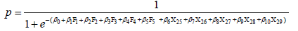(10)

In practical applications, 0.5 is generally used as the dividing line of the dependent variable to take 0 or 1. If the P value is closer to 0, the better the credit, the smaller the default rate, the more close to 1, the worse the credit, the higher the default rate.

4.3. Logistic Regression Analysis

4.3.1. Statistical Test of the Model

After screening, 4 variables were retained, namely profitability F1, solvency F2, liquidity F3 and Industry development prospects X26 (Table 3 and Table 4).

Test the goodness of fit of the model by Hosmer and Lemeshow test, the test results show that the chi-square value is 6.902, P value is 0.547, greater than the significance level, does not reject the original hypothesis, the model is estimated to fit the data at an acceptable level. In addition, the results from Table 3 can be seen that the model of Cox & Snell R side is 0.559 and Nagelkerke R Square is 0.746, through the above analysis can be seen that the model goodness of fit better.

4.3.2. Coefficient Estimation and Interpretation of the Model

In Table 3, the SME loan risk assessment model can be obtained by substituting factor:

$p=\frac{1}{1+{\text{e}}^{-\left(-4.565-3.463F_1-2.330F_2-3.327F_3+1.698X_{26}\right)}}$ (11)

Table 3. Hosmer and Lemeshow inspection.

Table 4. Variable filter tables.

Substituting p in Equation (9) includes:

$odds={\text{e}}^{-4.565-3.463F_1-2.330F_2-3.327F_3+1.698X_{26}}$ (12)

As can be seen from the formula (10), the occurrence ratio also changes when the independent variable changes. The ratio of the occurrence of the change to the occurrence before the change is known as the rate of occurrence, so that the self-variable can be used to interpret the occurrence ratio.

$\frac{odds}{odd{s}_1}=\frac{{\text{e}}^{-4.565-3.463\left(F_1+1\right)-2.330F_2-3.327F_3+1.698X_{26}}}{{\text{e}}^{-4.565-3.463F_1-2.330F_2-3.327F_3+1.698X_{26}}}={\text{e}}^{-3.463}$ (13)

From the formula (11) It can be seen that: when the rate of occurrence is greater than 1 o’clock, the independent variable has a positive effect on the occurrence probability of the event, and when the rate of occurrence is less than 1 o’clock, the independent variable has a reverse effect on the occurrence probability The ratio of the last remaining 4 variables (F1, F2, F3, X26) in the logistic model is calculated, as shown in Table 5.

As seen from Table 4, profitability F1, solvency F2 and liquidity F3 have a reverse effect on the probability of default in enterprises, and the development prospect of the industry X26 has a positive impact on the probability of the occurrence of default.

4.4. Model Evaluation and Predictive Ability Analysis

The usual statistical inference hypothesis testing two types of errors may occur, the Type I error may cause the loss of bank interest and loan principal; Type II error may cause the bank not to credit the “good” corporate loans and lose some interest income. So in practice, you should minimize the probability of the first type of error occurring. This article analyzes the first and second classes model error rates by selecting different default demarcation point. As can be seen from Table 6, with the gradual increase of the default demarcation point, the probability of the first type of error gradually increases, the probability of the second type of error gradually decreases, the impact rate of the first type of error is more serious, so on the premise of low miscalculation rate of the first type of error and strong overall predictive ability of the model, When the credit risk of commercial banks is evaluated by using logit model, 0.5 is usually the boundary point, which is consistent with the traditional boundary point selection standard. At this boundary point, the first type of error rate is 3.3%, the second type error rate is 10%, the first class error rate is relatively low, the overall accuracy rate of the model is 93.3%, the prediction effect is more ideal.

4.5. Logistic Regression Model Test

Inspection of the credit risk assessment model developed above data test sample set, enter data into the formula, we can obtain the probability of default, and then compared with the default cut-off point, which can evaluate credit risks. Table 7 shows, in the default cut-off point of 0.5, the correct model was 90%, slightly lower than the 93.3% obtained by modeling the sample, which have a certain relationship with the test sample size of the sample set, but in general, prediction model or ideal.

5. Conclusion

Through analysis, it is concluded that the 3 financial index variables of profitability F1, solvency F2 and liquidity F3 have a negative effect on the probability of default. This non-financial index has a positive effect on the probability of default of the enterprise by analyzing the X26 of the industry development. The

Table 5. Variable occurrence ratio statistics.

Table 6. Judgment results of different default cut-off points.

Table 7. Test results statistics.

overall prediction accuracy rate of the Logit model for SME credit risk assessment is 93.4% for the selected sample group, and 90% for the test sample group. Generally speaking, the prediction effect of the model is better. The model can be used to measure the credit risk of SMEs in China and the actual operation of commercial banks. It has a good reference meaning. In view of the confidentiality of the information of commercial banks, the acquisition of sample data is difficult, resulting in that the selection of sample size is small, the future research can appropriately expand the sample scale, at the same time, the introduction of macro-economic variables, industrial variables and other non-financial factors for analysis, in order to further improve the accuracy and applicability of the model.

Conflicts of Interest

The authors declare no conflicts of interest.

References

[1]	Altman, E.I. and Sabato, G. (2007) Modeling Credit Risk for SMEs: Evidence from the US Market. Journal of Financial Services Research, 43, 332-357.
[2]	Altman, E.I., Sabato, G. and Wilson, N. (2008) The Value of Qualitative Information in SME Risk Management. Journal of Financial Services Research, 40, 15-55.
[3]	Koyuncugil, A.S. (2012) Financial Early Warning System Model and Data Mining Application for Risk Detection. Expert Systems with Applications, 39, 6238-6253. https://doi.org/10.1016/j.eswa.2011.12.021
[4]	Yang, Y. (2009) Research on Credit Risk Assessment of SMEs in China. Financial Forum, No. 3, 69-73.
[5]	Shi, X. (2008) Application of BP Neural Network in Credit Risk Assessment of Chenghai Credit Union. Consumer Guide, No. 21, 104.
[6]	Zhou, M. (2010) The Way to Solve the Financing Difficulties of Small and Medium-Sized Enterprises. Contemporary Financiers, No. 2-3, 88-89
[7]	Liu, C. and Liu, X. (2012) SME Credit Risk Assessment Based on Credibility Theory. Technical Economics and Management Research, 10, 3-7.
[8]	Guo, S. (2014) Reflections on the Financial Risk Early-Warning of SMEs in the Context of Business Transformation of Commercial Banks. Business Times, No. 7, 74-75.
[9]	Cui, L. (2015) Dennis International Reference and Inspiration SME Credit Risk Prevention and Control. Study Financial and Economic, No. S1, 50-53.
[10]	Wu, J. (2016) Construction of Credit Risk Evaluation Index System for SMEs. Financial Communications, No. 26, 102-104.