A Characterization of Besov Spaces of Para-Accretive Type and Its Application

Junxian Li, Kunchuan Wang^*

Department of Applied Mathematics, National Dong Hwa University, Hualien.

DOI: 10.4236/am.2017.84046                

Abstract

There are two folds in this article. One fold is to characterize the Besov spaces of para-accretive type , which reduces to the classical Besov spaces when the para-accretive function is constant, by using a discrete Calderón-type reproducing formula and Plancherel-Pôlya-type inequality associated to a para-accretive function b in Rⁿ. The other is to show that a generalized singular integral operator T with extends to be bounded from for and , where ε is the regularity exponent of the kernel of T.

Keywords

Besov Space, Calderón Reproducing Formula, Para-Accretive Function, Tb Theorem, Triebel-Lizorkin Space

1. Introduction

Since Calderón and Zygmund developed the theory of singular integral opera- tors in the fifties in last century, there have been lots of eagerness to generalize the theory in various ways. One kind of interest is to consider the boundedness of such operators on Hardy spaces, Triebel-Lizorkin spaces or Besov spaces (cf. [1] - [13] ). The other interests include considering non-convolution operators such as the Calderón commutators (e.g. the $T1$ and $Tb$ theorems [14] [15] ) or investigating operator-valued kernels (cf. [16] [17] [18] ).

The remarkable $T1$ theorem given by David and Journé [14] provides a general criterion for the $L^2$ -boundedness of these generalized singular integral operators. Frazier, Torres, and Weiss [4] considered the $T1$ theorem on Triebel-Lizorkin spaces ${\stackrel{\dot{}}{F}}_p^{\alpha \mathrm{,}q}$ , which include the classical $L^p$ spaces for $1<p<\infty$ and Hardy spaces $H^p$ for $0<p\le 1$ , under the hypothesis $T{x}^{\gamma }=T^{*}{x}^{\gamma }=0$ for a certain condition on $\gamma$ . Afterward of of authors of the current paper extended the boundedness of singular integral operators acting on ${\stackrel{\dot{}}{F}}_p^{\alpha \mathrm{,}q}$ to more relaxed restriction on $T{x}^{\gamma }$ and $T^{\mathrm{<mo>\; *\; </mo>}}{x}^{\gamma }$ , see [12] [13] for details.

The $Tb$ theorem for spaces of homogeneous type introduced by Coifman and Weiss was proved in [15] . If function 1 in the $T1$ theorem is replaced by an accretive function, a bounded complex-valued function $b$ satisfying $0<\delta \le \mathrm{Re}b\left(x\right)$ almost everywhere, McIntosh and Meyer [10] showed the $L^2$ boundedness of the Cauchy integral on all Lipschitz curves. David, Journé, and Semmes [15] gave more general conditions on $L^{\infty }$ functions, therefore one said para-accretive functions, and proved a new $Tb$ theorem by substituting function 1 for para-accretive functions. It was also shown that if $Tb$ theorem holds for a bounded function $b$ , then $b$ is necessarily para-accretive in [15] .

In 2009, Lin and Wang [8] used a discrete Calderón-type reproducing formula and Plancherel-Pôlya-type inequality to characterize homogeneous Triebel- Lizorkin spaces of para-accretive type ${\stackrel{\dot{}}{F}}_{b\mathrm{,}p}^{\alpha \mathrm{,}q}$ . A necessary and sufficient condition of singular integral operators which is bounded from ${\stackrel{\dot{}}{F}}_{\mathrm{1,}p}^{\mathrm{0,}q}$ to ${\stackrel{\dot{}}{F}}_{b\mathrm{,}p}^{\mathrm{0,}q}$ ,

$\frac{n}{n+\epsilon }<p\le 1$ and $\frac{n}{n+\epsilon }<q\le 2$ with the regularity exponent $\epsilon$ of the kernel, is also derived in [8] . In this article, we study the ${\stackrel{\dot{}}{B}}_{\mathrm{1,}p}^{\mathrm{0,}q}-{\stackrel{\dot{}}{B}}_{b\mathrm{,}p}^{\mathrm{0,}q}$ boundedness of singular integral operators for wider ranges of $\max \left\{\frac{n}{n+\epsilon },\frac{n}{n+\alpha +\epsilon }\right\}<p<\infty$ and $0<q\le \infty$ .

One begins by recalling some basic results about Calderón-Zygmund operator theory. As usual, ${\mathcal{D}}_c\left({ℝ}^n\right)$ denotes the set of $C^{\infty }$ functions with compact support and $\mathcal{S}\left({ℝ}^n\right)$ denotes the Schwartz class.

Definition 1.1. We say that $T$ is a singular integral operator, denoted by $T\in SIO\left(\epsilon \right)$ , if $T$ is a continuous linear operator from $\mathcal{S}\left({ℝ}^n\right)$ into its dual associated to a kernel $K\left(x\mathrm{,}y\right)$ , a continuous function defined on ${ℝ}^n\times {ℝ}^n\backslash \left\{x=y\right\}$ , satisfying the following conditions: there exist constants $C>0$ and $0<\epsilon \le 1$ such that

$\left|K\left(x,y\right)\right|\le C\frac{1}{{\left|x-y\right|}^n}\text{forall}x\ne y$ (1)

$\left|K\left(x,y\right)-K\left(x^{\prime },y\right)\right|\le C\frac{{\left|x-x^{\prime }\right|}^{\epsilon }}{{\left|x-y\right|}^{n+\epsilon }}\text{forall}x\mathrm{,}{x}^{\prime }\mathrm{,}y\in {ℝ}^n\text{with}\left|x-x^{\prime }\right|\le \frac{\left|x-y\right|}{2}$ (2)

$\left|K\left(x\mathrm{,}y\right)-K\left(x\mathrm{,}{y}^{\prime }\right)\right|\le C\frac{{\left|y-y^{\prime }\right|}^{\epsilon }}{{\left|x-y\right|}^{n+\epsilon }}\text{forall}y\mathrm{,}{y}^{\prime }\mathrm{,}x\in {ℝ}^n\text{with}\left|y-y^{\prime }\right|\le \frac{\left|x-y\right|}{2}$ (3)

Moreover, the operator $T$ can be represented by

$\langle Tf\mathrm{,}g\rangle \mathrm{<mo>\; =\; </mo>}{\displaystyle {\int }_{{ℝ}^n}}{\displaystyle {\int }_{{ℝ}^n}K\left(x\mathrm{,}y\right)f\left(y\right)g\left(x\right)\text{d}y\text{d}x}$ (4)

for all $f,g\in {\mathcal{D}}_c\left({ℝ}^n\right)$ with $\text{supp}\left(f\right)\cap \text{supp}\left(g\right)=\varnothing$ .

We say that a singular integral operator is a Calderón-Zygmund operator if it can be extended to a bounded operator on $L^2\left({ℝ}^n\right)$ . Coifman and Meyer [19] showed that every Calderón-Zygmund operator is bounded on $L^p$ for $1<p<\infty$ .

A locally integrable function defined on ${ℝ}^n$ belongs to $BMO$ if it satisfies

${\Vert f\Vert }_{{}_{BMO}}:=\underset{Q}{\sup }\frac{1}{\left|Q\right|}{\displaystyle {\int }_Q\left|f\left(x\right)-f_Q\right|\text{d}x}<\infty$ (5)

where the supremum is taken over all cubes $Q\subseteq {ℝ}^n$ whose sides are parallel to the axes and $f_Q\mathrm{<mo>\; =\; </mo>}\frac{1}{\left|Q\right|}{\displaystyle {\int }_{Q}f\left(x\right)\text{d}x}$ . Note that these cubes need not be dyadic. For $f\in {\mathcal{D}}_c\left({ℝ}^n\right)$ , $t>0$ and $z\in {ℝ}^n$ , let $f_t^z\left(x\right):=t^{n}f\left(\left(x-z\right)/t\right)$ .

Definition 1.2. Let $T:\mathcal{S}\left({ℝ}^n\right)\mapsto {\mathcal{S}}^{\prime }\left({ℝ}^n\right)$ be a continuous linear operator. $T$ is called to have the weak boundedness property, denoted by $T\in WBP$ , if for every bounded subset $B$ of ${\mathcal{D}}_c\left({ℝ}^n\right)$ , there is a constant $C>0$ such that

$\left|\langle T{f}_t^z,g_t^z\rangle \right|\le C{t}^{-n}$ (6)

for all $f$ and $g$ in $\mathcal{B}$ , $z\in {ℝ}^n$ , and $t>0$ .

David and Journé [14] gave a general criterion for the $L^2$ boundedness of singular integral operators as follows:

Proposition 1.3 ($T1$ theorem for L²) Suppose that $T\in SIO\left(\epsilon \right)$ for some $\epsilon >0$ and $T^{\mathrm{<mo>\; *\; </mo>}}$ denotes its transpose. Then $T$ extends to be bounded on $L^2$ if and only if $T1\in BMO$ , $T^{\mathrm{<mo>\; *\; </mo>}}1\in BMO$ , and $T\in WBP$ .

Before stating the $Tb$ theorem of David, Journé and Semmes [15] , one recalls some definitions. Let $C_0^{\eta }$ denote the space of continuous functions $f$ with compact support such that

${\Vert f\Vert }_{\eta }:=\underset{x\ne y}{\sup }\frac{\left|f\left(x\right)-f\left(y\right)\right|}{{\left|x-y\right|}^{\eta }}<\infty$ (7)

Definition 1.4. A bounded complex-valued function $b$ defined on ${ℝ}^n$ is said to be para-accretive if there exist constants $C,\gamma >0$ such that, for all cubes $Q\subseteq {ℝ}^n$ , there is a subcube $Q^{\prime }\subseteq Q$ with $\gamma \left|Q\right|\le \left|Q^{\prime }\right|$ satisfying

$\frac{1}{\left|Q\right|}\left|{\displaystyle {\int }_{Q^{\prime }}b\left(x\right)\text{d}x}\right|\ge C>0$ (8)

Definition 1.5. Suppose $b_1$ and $b_2$ are bounded complex-valued functions whose inverses are also bounded. A generalized singular integral operator is a continuous linear operator $T$ from $b_1{C}_0^{\eta }$ into ${\left(b_2{C}_0^{\eta }\right)}^{\prime }$ , $\eta >0$ , for which the associated kernel $K\left(x\mathrm{,}y\right)$ satisfies inequalities (1)-(3) such that, for all $f$ , $g\in C_0^{\eta }$ with $\text{supp}\left(f\right)\cap \text{supp}\left(g\right)=\varnothing$ ,

$\langle T{b}_{1}f,b_{2}g\rangle ={\displaystyle {\int }_{{ℝ}^n}}{\displaystyle {\int }_{{ℝ}^n}g\left(x\right)b_2\left(x\right)K\left(x,y\right)b_1\left(y\right)f\left(y\right)\text{d}x\text{d}y}$ (9)

Such an operator $T$ is written as $T\in GSIO\left(\epsilon \right)$ , where $\epsilon$ is the regularity exponent of $K\left(x\mathrm{,}y\right)$ in Definition 1.1.

Denote $M_b$ the multiplication operator by $b$ ; that is, $M_{b}f=bf$ . David, Journé and Semmes [15] proved the following $Tb$ theorem.

Proposition 1.6. ( $Tb$ theorem for $L^2$ ) Suppose that $b_1$ and $b_2$ are para- accretive functions and $T\in GSIO\left(\epsilon \right)$ . Then $T$ extends to be bounded on $L^2$ if and only if (1) $T{b}_1\in BMO$ , (2) $T^{\mathrm{<mo>\; *\; </mo>}}{b}_2\in BMO$ , and (3) $M_{b_2}T{M}_{b_1}\in WBP$ .

Later on Lin and Wang gave the following result. For any $x\in ℝ$ , let $\left[x\right]$ denote the integer part of $x$ and $x^{*}=x-\left[x\right]$ . For $0<p,$ $q\le \infty$ , $J=n/\min \left(1,p,q\right)$ .

Proposition 1.7. ( [8] ) Assume that $b$ is a para-accretive function. Let $T\in GSIO\left(\epsilon \right)$ and $M_{b}T{M}_b\in WBP$ for some $\epsilon >J^{*}$ . For $\alpha \in \left(-\epsilon \mathrm{,}\epsilon \right)$ , $\max \left\{\frac{n}{n+\epsilon },\frac{n}{n+\epsilon +\alpha }\right\}<p<\infty$ and $\max \left\{\frac{n}{n+\epsilon },\frac{n}{n+\epsilon +\alpha }\right\}<q\le \infty$ , if $Tb=T^{*}b=0$ , then $T$ extends to a bounded linear operator from ${\stackrel{\dot{}}{F}}_{\mathrm{1,}p}^{\alpha \mathrm{,}q}$ to ${\stackrel{\dot{}}{F}}_{b\mathrm{,}p}^{\alpha \mathrm{,}q}$ .

The main purpose and methods used in this paper is related to a $Tb$ theorem in Besov spaces of para-accretive type ${\stackrel{\dot{}}{B}}_{b\mathrm{,}p}^{\mathrm{0,}q}$ , which was introduced by Han [20] for $p$ , $q>1$ , by Deng and Yang [21] for $p$ , $q\le 1$ , denoted as $b^{-1}{\stackrel{\dot{}}{B}}_p^{\mathrm{0,}q}$ . Once one has an approximation to the identity, a Plancherel-Pôlya-type inequality follows immediately. For the terminology used in the rest of this section, see Section 2 for details.

Theorem 1.8 (Plancherel-Polya-type inequality) Let $\alpha \in \left(-\epsilon ,\epsilon \right),$ $\max \left\{\frac{n}{n+\epsilon },\frac{n}{n+\epsilon +\alpha }\right\}<p<\infty$ and $0<q\le \infty$ . Suppose that $S={\left\{S_k\right\}}_{k\in \mathbb{Z}}$ is an approximation to the identity defined in Definition 2.1 and $V={\left\{V_k\right\}}_{k\in \mathbb{Z}}$ is another approximation to the identity with the same properties as the ${\left\{S_k\right\}}_{k\in \mathbb{Z}}$ . Set $D_k=S_k-S_{k-1}$ and $E_k=V_k-V_{k-1}$ .

a) For all $f\in {\left(b{\mathcal{M}}^{\left(\beta ,\gamma \right)}\right)}^{\prime }$ , if ${\left\{{\displaystyle {\sum }_k}{\Vert {\displaystyle {\sum }_{Q_k}}{2}^{k\alpha }{{\displaystyle \sup }}_{z\in Q_k}\left|E_{k}bf\left(z\right)\right|{\chi }_{Q_k}\Vert }_p^q\right\}}^{1/q}$ is finite then

#Math_175# (10)

b) For all $f\in {\left({\mathcal{M}}^{\left(\beta ,\gamma \right)}\right)}^{\prime }$ , if ${\left\{{\displaystyle {\sum }_k}{\Vert {\displaystyle {\sum }_{Q_k}}{2}^{k\alpha }{{\displaystyle sup}}_{z\in Q_k}\left|E_{k}f\left(z\right)\right|{\chi }_{Q_k}\Vert }_p^q\right\}}^{1/q}$ is finite then

${\left\{{\displaystyle \underset{k}{\sum }}{\Vert {\displaystyle \underset{Q_k}{\sum }}{2}^{k\alpha }\underset{z\in Q_k}{\sup }\left|E_{k}f\left(z\right)\right|{\chi }_{Q_k}\Vert }_p^q\right\}}^{1/q}\approx {\left\{{\displaystyle \underset{k}{\sum }}{\Vert {\displaystyle \underset{Q_k}{\sum }}{2}^{k\alpha }\underset{z\in Q_k}{\inf }\left|D_{k}f\left(z\right)\right|{\chi }_{Q_k}\Vert }_p^q\right\}}^{1/q}$ (11)

Now it is ready to define a class of the homogeneous Besov spaces associated to para-accretive functions.

Definition 1.9. Let $S={\left\{S_k\right\}}_{k\in \mathbb{Z}}$ be an approximation to the identity defined in Definition 2.1 and set $D_k=S_k-S_{k-1}$ for $k\in \mathbb{Z}$ as before. For $\alpha \in \left(-\epsilon \mathrm{,}\epsilon \right)$ , $\max \left\{\frac{n}{n+\epsilon },\frac{n}{n+\alpha +\epsilon }\right\}<p<\infty$ , and $0<q\le \infty$ , the homogeneous Besov spaces of para-accretive type ${\stackrel{\dot{}}{B}}_{b\mathrm{,}p}^{\alpha \mathrm{,}q}$ is the collection of $f\in {\left(b{\mathcal{M}}^{\left(\beta ,\gamma \right)}\right)}^{\prime }$ such that

${\Vert f\Vert }_{{\stackrel{\dot{}}{B}}_{b,p}^{\alpha ,q}\left(S\right)}={\left\{{\displaystyle \underset{k}{\sum }}{2}^{k\alpha q}{\Vert D_{k}bf\left(x\right)\Vert }_p^q\right\}}^{1/q}<\infty$ (12)

From Theorem 1.8, one can check that Definition 1.9 is independent of choices of approximations to the identity. As an application, one has the follow- ing.

Theorem 1.10. (Reduced Tb theorem for Besov spaces of para-accretive type) Assume that $b$ is a para-accretive function. Let $T\in GSIO\left(\epsilon \right)$ and $M_{b}T{M}_b\in WBP$ for some $\epsilon >J^{*}$ . For $\alpha \in \left(-\epsilon \mathrm{,}\epsilon \right)$ , $\max \left\{\frac{n}{n+\epsilon },\frac{n}{n+\alpha +\epsilon }\right\}<p<\infty$ and $0<q\le \infty$ , if $Tb=T^{*}b=0$ then $T$ extended to a bounded linear operator from ${\stackrel{\dot{}}{B}}_{\mathrm{1,}p}^{\alpha \mathrm{,}q}$ to ${\stackrel{\dot{}}{B}}_{b\mathrm{,}p}^{\alpha \mathrm{,}q}$ .

The proof of this main result is based on the discrete Calderón-type reproduc- ing formula [5] , a characterization of Besov spaces ${\stackrel{\dot{}}{B}}_{b\mathrm{,}p}^{\alpha \mathrm{,}q}$ , and a Plancherel- Pôlya-type inequality.

This paper is organized as follows. In Section 2, one gives some preliminaries. Then one states and proves a Plancherel-Pôlya-type inequality in Section 3. Then one uses a Plancherel-Pôlya-type inequality to show norm equivalence between Besov space ${\stackrel{\dot{}}{B}}_{b\mathrm{,}p}^{\alpha \mathrm{,}q}$ and its corresponding sequence space ${\stackrel{\dot{}}{b}}_p^{\alpha \mathrm{,}q}$ in Section 4. Finally one proves reduced $Tb$ theorem for Besov spaces of para-accretive type in Section 5. Through the paper, one uses $Q$ to denote a dyadic cube in ${ℝ}^n$ , $j\wedge k$ denotes the minimum of $j$ and $k$ and uses $C$ to denote a positive constant independent of the main variables, which may vary from line to line. Also $A\approx B$ means that there exist two positive constants $c_1$ and $c_2$ so that $c_{1}A\le B\le c_{2}A$ .

2. Preliminaries

Recall the definition of approximation to the identity associated to a para- accretive function and a related Calderón reproducing formula generated by such an approximation to the identity, and start with “test functions’’ given by Han [20] . Fix two exponents $0<\beta \le 1$ and $\gamma >0$ . Suppose that $b$ is a para- accretive function. A function $f$ defined on ${ℝ}^n$ is said to be a test function of type $\left(\beta \mathrm{,}\gamma \mathrm{,}b\right)$ centered at $x_0\in {ℝ}^n$ with width $d>0$ if

$\left|f\left(x\right)\right|\le C\frac{d^{\gamma }}{{\left(d+\left|x-x_0\right|\right)}^{n+\gamma }}$ (13)

$\left|f\left(x\right)-f\left(x^{\prime }\right)\right|\le C{\left(\frac{\left|x-x^{\prime }\right|}{d+\left|x-x_0\right|}\right)}^{\beta }\frac{d^{\gamma }}{{\left(d+\left|x-x_0\right|\right)}^{n+\gamma }}\text{for}\left|x-x^{\prime }\right|\le \frac{d+\left|x-x_0\right|}{2}$ (14)

${\displaystyle {\int }_{{ℝ}^n}f\left(x\right)b\left(x\right)\text{d}x}=0$ (15)

Denote by ${\mathcal{M}}^{\left(\beta \mathrm{,}\gamma \mathrm{,}b\right)}\left(x_0\mathrm{,}d\right)$ the collection of all test functions of type $\left(\beta \mathrm{,}\gamma \mathrm{,}b\right)$ centered at $x_0\in {ℝ}^n$ with width $d>0$ . For $f\in {\mathcal{M}}^{\left(\beta ,\gamma ,b\right)}\left(x_0,d\right)$ , the norm of $f$ in ${\mathcal{M}}^{\left(\beta \mathrm{,}\gamma \mathrm{,}b\right)}\left(x_0\mathrm{,}d\right)$ is defined by

${\Vert f\Vert }_{{\mathcal{M}}^{\left(\beta ,\gamma ,b\right)}\left(x_0,d\right)}:=\inf \left\{C:\left(13\right)\text{and}\left(14\right)\text{hold}\right\}$ (16)

We denote ${\mathcal{M}}^{\left(\beta \mathrm{,}\gamma \mathrm{,}b\right)}\left(\mathrm{0,1}\right)$ simply by ${\mathcal{M}}^{\left(\beta \mathrm{,}\gamma \mathrm{,}b\right)}$ .

It is clear that ${\mathcal{M}}^{\left(\beta \mathrm{,}\gamma \mathrm{,}b\right)}$ is a Banach space under the norm ${\Vert f\Vert }_{{\mathcal{M}}^{\left(\beta \mathrm{,}\gamma \mathrm{,}b\right)}}$ . Write

$b{\mathcal{M}}^{\left(\beta ,\gamma ,b\right)}:=\left\{f|f=bg\text{for}\text{some}g\in {\mathcal{M}}^{\left(\beta \mathrm{,}\gamma \mathrm{,}b\right)}\right\}$ (17)

If $f\in b{\mathcal{M}}^{\left(\beta \mathrm{,}\gamma \mathrm{,}b\right)}$ and $f=bg$ for $g\in {\mathcal{M}}^{\left(\beta \mathrm{,}\gamma \mathrm{,}b\right)}$ , then the norm of $f$ is defined by ${\Vert f\Vert }_{b{\mathcal{M}}^{\left(\beta ,\gamma ,b\right)}}:={\Vert g\Vert }_{{\mathcal{M}}^{\left(\beta ,\gamma ,b\right)}}$ . As usual, one uses ${\left({\mathcal{M}}^{\left(\beta \mathrm{,}\gamma \mathrm{,}b\right)}\right)}^{\prime }$ and ${\left(b{\mathcal{M}}^{\left(\beta ,\gamma ,b\right)}\right)}^{\prime }$ to denote the dual spaces of ${\mathcal{M}}^{\left(\beta \mathrm{,}\gamma \mathrm{,}b\right)}$ and $b{\mathcal{M}}^{\left(\beta \mathrm{,}\gamma \mathrm{,}b\right)}$ , respectively. Use $\langle h\mathrm{,}f\rangle$ to denote the natural pairing of elements $h\in {\left({\mathcal{M}}^{\left(\beta \mathrm{,}\gamma \mathrm{,}b\right)}\right)}^{\prime }$ and

$f\in {\mathcal{M}}^{\left(\beta \mathrm{,}\gamma \mathrm{,}b\right)}\mathrm{.}$ It is easy to check that for any $x_0\in {ℝ}^n$ and $d>0,$ ${\mathcal{M}}^{\left(\beta ,\gamma ,b\right)}\left(x_0,d\right)={\mathcal{M}}^{\left(\beta ,\gamma ,b\right)}$ with equivalent norms. Thus, given $h\in \left({\mathcal{M}}^{\left(\beta ,\gamma ,b\right)}\right)$ , $\langle h\mathrm{,}f\rangle$ is well defined for all $f\in {\mathcal{M}}^{\left(\beta ,\gamma ,b\right)}\left(x_0,d\right)$ with any $x_0\in {ℝ}^n$ and $d>0$ .

In order to state the Calderón reproducing formula, one also needs an approximation to the identity (cf. [7] [15] [20] ).

Definition 2.1. Let $b$ be a para-accretive function. A sequence of linear operators ${\left\{S_k\right\}}_{k\in \mathbb{Z}}$ is called an approximation to the identity associated to $b$ if the kernels $S_k\left(x,y\right)$ of $S_k$ are functions from ${ℝ}^n\times {ℝ}^n$ into $ℂ$ such that there exist constant $C$ and some $0<\epsilon \le 1$ satisfying, for all $k\in \mathbb{Z}$ and all $x,x^{\prime },y$ , and $y^{\prime }\in {ℝ}^n$ ,

1) $\left|S_k\left(x,y\right)\right|\le C\frac{2^{-k\epsilon }}{{\left(2^{-k}+\left|x-y\right|\right)}^{n+\epsilon }},$

2) $\left|S_k\left(x,y\right)-S_k\left(x^{\prime },y\right)\right|\le C{\left(\frac{\left|x-x^{\prime }\right|}{2^{-k}+\left|x-y\right|}\right)}^{\epsilon }\frac{2^{-k\epsilon }}{{\left(2^{-k}+\left|x-y\right|\right)}^{n+\epsilon }},$

for $\left|x-x^{\prime }\right|\le \frac{1}{2}\left(2^{-k}+\left|x-y\right|\right)$ ,

3) $\left|S_k\left(x,y\right)-S_k\left(x,y^{\prime }\right)\right|\le C{\left(\frac{\left|y-y^{\prime }\right|}{2^{-k}+\left|x-y\right|}\right)}^{\epsilon }\frac{2^{-k\epsilon }}{{\left(2^{-k}+\left|x-y\right|\right)}^{n+\epsilon }},$

for $\left|y-y^{\prime }\right|\le \frac{1}{2}\left(2^{-k}+\left|x-y\right|\right)$ ,

4) $\begin{array}{l}\left|\left[S_k\left(x,y\right)-S_k\left(x,y^{\prime }\right)\right]-\left[S_k\left(x^{\prime },y\right)-S_k\left(x^{\prime },y^{\prime }\right)\right]\right|\\ \le C{\left(\frac{\left|x-x^{\prime }\right|}{2^{-k}+\left|x-y\right|}\right)}^{\epsilon }{\left(\frac{\left|y-y^{\prime }\right|}{2^{-k}+\left|x-y\right|}\right)}^{\epsilon }\frac{2^{-k\epsilon }}{{\left(2^{-k}+\left|x-y\right|\right)}^{n+\epsilon }},\end{array}$

for $\left|x-x^{\prime }\right|\le \frac{1}{2}\left(2^{-k}+\left|x-y\right|\right)$ and $\left|y-y^{\prime }\right|\le \frac{1}{2}\left(2^{-k}+\left|x-y\right|\right),$

5) ${\displaystyle {\int }_{{ℝ}^n}{S}_k\left(x,y\right)b\left(y\right)\text{d}y}=1$ for all $k\in \mathbb{Z}$ and $x\in {ℝ}^n$ ,

6) ${\displaystyle {\int }_{{ℝ}^n}{S}_k\left(x,y\right)b\left(x\right)\text{d}x}=1$ for all $k\in \mathbb{Z}$ and $y\in {ℝ}^n$ .

The following discrete Calderón reproducing formulae were given in [5] .

Proposition 2.2. Suppose that $\left\{S_k\right\}$ is an approximation to the identity defined in Definition 2.1. Set $D_k=S_k-S_{k-1}$ . Then there exists a family of operators $\left\{{\mathcal{D}}_k\right\}$ with kernel ${\mathcal{D}}_k\left(x\mathrm{,}y\right)$ satisfying, for $0<{\epsilon }^{\prime }<\epsilon$ ,

$\left|{\mathcal{D}}_k\left(x,y\right)\right|\le C\frac{2^{-k{\epsilon }^{\prime }}}{{\left(2^{-k}+\left|x-y\right|\right)}^{n+{\epsilon }^{\prime }}}$ (18)

$\begin{array}{l}\left|{\mathcal{D}}_k\left(x\mathrm{,}y\right)-{\mathcal{D}}_k\left(x\mathrm{,}{y}^{\prime }\right)\right|\le C{\left(\frac{\left|y-y^{\prime }\right|}{2^{-k}+\left|x-y\right|}\right)}^{{\epsilon }^{\prime }}\frac{2^{-k{\epsilon }^{\prime }}}{{\left(2^{-k}+\left|x-y\right|\right)}^{n+{\epsilon }^{\prime }}}\\ \text{for}\left|y-y^{\prime }\right|\le \left(2^{-k}+\left|x-y\right|\right)/2\end{array}$ (19)

${\displaystyle {\int }_{{ℝ}^n}{\mathcal{D}}_k\left(x\mathrm{,}y\right)b\left(y\right)\text{d}y}=0\text{for}\text{all}k\in \mathbb{Z}\text{and}x\in {ℝ}^n$ (20)

${\displaystyle {\int }_{{ℝ}^n}{\mathcal{D}}_k\left(x\mathrm{,}y\right)b\left(x\right)\text{d}x}=0\text{for}\text{all}k\in \mathbb{Z}\text{and}y\in {\mathbb{Z}}^n$ (21)

such that,

$f\left(x\right)={\displaystyle \underset{k\in \mathbb{Z}}{\sum }}{\displaystyle \underset{Q}{\sum }{D}_{k}f\left(y_{{}_Q}\right)}{\displaystyle {\int }_{Q}b\left(x\right){\mathcal{D}}_k\left(y,x\right)b\left(y\right)\text{d}y}\text{forall}f\in {\left({\mathcal{M}}^{\left(\beta \mathrm{,}\gamma \mathrm{,}b\right)}\right)}^{\prime }$ (22)

and

$f\left(x\right)={\displaystyle \underset{k}{\sum }}{\displaystyle \underset{Q}{\sum }{D}_{k}bf\left(y_{{}_Q}\right){\displaystyle {\int }_Q{\mathcal{D}}_k\left(y,x\right)b\left(y\right)\text{d}y}}\text{forall}f\in {\left(b{\mathcal{M}}^{\left(\beta ,\gamma ,b\right)}\right)}^{\prime }$ (23)

where $Q$ are all dyadic cubes with the side length $2^{-k-N}$ for some fixed positive large integer $N$ and $y_{{}_Q}$ is any fixed point in $Q$ .

Note that $f\in {\left(b{\mathcal{M}}^{\left(\beta \mathrm{,}\gamma \mathrm{,}b\right)}\right)}^{\prime }$ if and only if $bf\in {\left({\mathcal{M}}^{\left(\beta ,\gamma ,b\right)}\right)}^{\prime }$ or equivalently, $f\in {\left({\mathcal{M}}^{\left(\beta ,\gamma ,b\right)}\right)}^{\prime }$ if and only if $b^{-1}f\in {\left({\mathcal{M}}^{\left(\beta ,\gamma ,b\right)}\right)}^{\prime }$ .

3. Plancherel-Pôlya-Type Inequalities

The classical Plancherel-Pôlya inequality has a long history and plays a central role in the theory of function spaces. Roughly speaking, if a tempered distribution $f$ in ${ℝ}^n$ , whose Fourier transform has compact support, then, by the Paley-Wiener theorem, it is an analytic function, or more precisely, entire analytic function of exponential type. The Plancherel-Pôlya inequality concludes that if $\left\{x_k\right\}$ is an appropriate set of points in ${ℝ}^n$ , e.g., lattice points, where the length of the mesh is sufficiently small, then

${\left({\displaystyle \underset{k=1}{\overset{\infty }{\sum }}{\left|f\left(x_k\right)\right|}^p}\right)}^{1/p}\approx {\Vert f\Vert }_p$ (24)

for all $0<p\le \infty$ with a modification if $p=\infty$ . The Fourier transform is the basic tool to prove such an inequality. See [22] for more details.

For any cube $Q$ and $\lambda >0$ , one denotes by $\lambda Q$ the cube concentric with $Q$ whose each edge is $\lambda$ times as long. A generalized Plancherel-Pôlya-type inequality for Triebel-Lizorkin spaces was given in [8] . In this section, one proves the following Plancherel-Pôlya-type inequalities in Besov sense.

Proof of Theorem 1.8. By Proposition 2.2, $f$ can be written as

$f\left(x\right)={\displaystyle \underset{k}{\sum }}{\displaystyle \underset{Q_k}{\sum }{D}_{k}bf\left(y_{Q_k}\right)}{\displaystyle {\int }_{Q_k}}{\mathcal{D}}_k\left(y,x\right)b\left(y\right)\text{d}y$ (25)

where $y_{Q_k}$ is any fixed point in $Q_k$ . To estimate

$E_{j}bf\left(x\right)={\displaystyle \underset{k}{\sum }}{\displaystyle \underset{Q_k}{\sum }{D}_{k}bf\left(y_{Q_k}\right)}{\displaystyle {\int }_{Q_k}}{E}_{j}b{\mathcal{D}}_k\left(y,\cdot \right)\left(x\right)b\left(y\right)\text{d}y$ (26)

using the inequality (see [7] )

$\left|E_{j}b{\mathcal{D}}_k\left(y,\cdot \right)\left(x\right)\right|=\left|{\displaystyle {\int }_{{ℝ}^n}{E}_j\left(x,z\right)b\left(z\right){\mathcal{D}}_k\left(y,z\right)\text{d}z}\right|\le C{2}^{-\left|j-k\right|{\epsilon }^{″}}\frac{2^{-\left(j\wedge k\right){\epsilon }^{\prime }}}{{\left(2^{-\left(j\wedge k\right)}+\left|x-y\right|\right)}^{n+{\epsilon }^{\prime }}}$ (27)

where ${\epsilon }^{\prime }$ and ${\epsilon }^{″}$ are close enough to $\epsilon$ and satisfy $\left|\alpha \right|<{\epsilon }^{″}<{\epsilon }^{\prime }<\epsilon$ , one obtains

$\begin{array}{c}\left|E_{j}bf\left(x\right)\right|\le C{\displaystyle \underset{k}{\sum }}{\displaystyle \underset{Q_k}{\sum }}\left|D_{k}bf\left(y_{Q_k}\right)\right|{\displaystyle {\int }_{Q_k}}{2}^{-\left|j-k\right|{\epsilon }^{″}}\frac{2^{-\left(j\wedge k\right){\epsilon }^{\prime }}}{{\left(2^{-\left(j\wedge k\right)}+\left|x-y\right|\right)}^{n+{\epsilon }^{\prime }}}\text{d}y\\ \le C{\displaystyle \underset{k}{\sum }}{\displaystyle \underset{Q_k}{\sum }}{2}^{-\left|j-k\right|{\epsilon }^{″}}{2}^{-kn}\frac{2^{-\left(j\wedge k\right){\epsilon }^{\prime }}}{{\left(2^{-\left(j\wedge k\right)}+\left|x-y_{Q_k}\right|\right)}^{n+{\epsilon }^{\prime }}}\left|D_{k}bf\left(y_{Q_k}\right)\right|\end{array}$ (28)

Thus,

$\underset{z\in Q_j}{\sup }\left|E_{j}bf\left(z\right)\right|{\chi }_{Q_j}\left(x\right)\le C{\displaystyle \underset{k}{\sum }}{\displaystyle \underset{Q_k}{\sum }}{2}^{-\left|j-k\right|{\epsilon }^{″}}{2}^{-kn}\frac{2^{-\left(j\wedge k\right){\epsilon }^{\prime }}}{{\left(2^{-\left(j\wedge k\right)}+\left|x-y\right|\right)}^{n+{\epsilon }^{\prime }}}\left|D_{k}bf\left(y_{Q_k}\right)\right|{\chi }_{Q_j}\left(x\right)$ (29)

For simplicity, let

$M_{f,V}:={\left\{{\displaystyle \underset{j}{\sum }}{\left[{\displaystyle \underset{Q_j}{\sum }}{\left({\left|Q_j\right|}^{-\alpha /n+1/p}\underset{z\in Q_j}{\sup }\left|E_{j}bf\left(z\right)\right|\right)}^p\right]}^{q/p}\right\}}^{1/q}$ (30)

First one considers the case for $p\le 1$ . In this case,

$\begin{array}{l}{M}_{f\mathrm{,}V}\le C{\left\{{\displaystyle \underset{j}{\sum }}\left[{\displaystyle \underset{k}{\sum }}{\displaystyle \underset{Q_j}{\sum }}{\displaystyle \underset{Q_k}{\sum }}{2}^{-k\alpha p}{2}^{j\alpha p}{2}^{-\left|j-k\right|p{\epsilon }^{″}}{2}^{-kpn}\left|Q_j\right|2^{kn}\times \frac{2^{-\left(j\wedge k\right)p{\epsilon }^{\prime }}}{{\left(2^{-\left(j\wedge k\right)}+\left|y_{Q_j}-y_{Q_k}\right|\right)}^{p\left(n+{\epsilon }^{\prime }\right)}}{2}^{k\alpha p}{\left|D_{k}bf\left(y_{Q_k}\right)\right|}^p\left|Q_k\right|\right]\right\}}^{1/q}\\ =C{\left\{{\displaystyle \underset{j}{\sum }}{\left[{\displaystyle \underset{k}{\sum }}{\displaystyle \underset{Q_j}{\sum }}{\displaystyle \underset{Q_k}{\sum }{2}^{-\left(k-j\right)\alpha p-\left|j-k\right|p{\epsilon }^{″}}{2}^{-kn\left(p-1\right)}}{\displaystyle {\int }_{Q_j}{\chi }_{{}_{Q_j}}\left(x\right)\text{d}x}\times \frac{2^{-\left(j\wedge k\right)p{\epsilon }^{\prime }}}{{\left(2^{-\left(j\wedge k\right)}+\left|y_{Q_j}-y_{Q_k}\right|\right)}^{p\left(n+{\epsilon }^{\prime }\right)}}{2}^{k\alpha p}{\left|D_{k}bf\left(y_{Q_k}\right)\right|}^p\left|Q_k\right|\right]}^{q/p}\right\}}^{1/q}\\ \le C{\left\{{\displaystyle \underset{j}{\sum }}{\left[{\displaystyle \underset{k}{\sum }}{\displaystyle \underset{Q_k}{\sum }{2}^{-\left(k-j\right)\alpha p-\left|j-k\right|p{\epsilon }^{″}}{2}^{-kn\left(p-1\right)}{2}^{k\alpha p}}{\left|D_{k}bf\left(y_{Q_k}\right)\right|}^p\left|Q_k\right|\times {\displaystyle {\int }_{{ℝ}^n}\frac{2^{-\left(j\wedge k\right)p{\epsilon }^{\prime }}}{{\left(2^{-\left(j\wedge k\right)}+\left|x-y_{Q_k}\right|\right)}^{p\left(n+{\epsilon }^{\prime }\right)}}\text{d}x}\right]}^{q/p}\right\}}^{1/q}\\ \le C{\left\{{\displaystyle \underset{j}{\sum }}{\left[{\displaystyle \underset{k}{\sum }}{2}^{-\left(k-j\right)\alpha p-\left|j-k\right|p{\epsilon }^{″}-kn\left(p-1\right)}{\displaystyle \underset{Q_k}{\sum }}{2}^{k\alpha p}{\left|D_{k}bf\left(y_{Q_k}\right)\right|}^p\left|Q_k\right|\right]}^{q/p}\right\}}^{1/q}\end{array}$

because we may choose ${\epsilon }^{\prime }$ so that

${\displaystyle {\int }_{{ℝ}^n}\frac{2^{-\left(j\wedge k\right)p{\epsilon }^{\prime }}}{{\left(2^{-\left(j\wedge k\right)}+\left|x-y_{Q_k}\right|\right)}^{p\left(n+{\epsilon }^{\prime }\right)}}\text{d}x}$ (31)

is finite. If $q\le p$ , then

$\begin{array}{c}{M}_{f,V}\le C{\left\{{\displaystyle \underset{j}{\sum }}{\displaystyle \underset{k}{\sum }{2}^{\left[-\left(k-j\right)\alpha p-\left|j-k\right|p{\epsilon }^{″}-kn\left(p-1\right)\right]q/p}{\left[{\displaystyle \underset{Q_k}{\sum }{2}^{k\alpha p}{\left|D_{k}bf\left(y_{Q_k}\right)\right|}^p\left|Q_k\right|}\right]}^{q/p}}\right\}}^{1/q}\\ \le C{\left\{{\displaystyle \underset{k}{\sum }}{\left[{\displaystyle \underset{Q_k}{\sum }{2}^{k\alpha p}{\left|D_{k}bf\left(y_{Q_k}\right)\right|}^p\left|Q_k\right|}\right]}^{q/p}\right\}}^{1/q}\end{array}$ (32)

Note that the last inequality is followed from

$\left(\underset{j}{\sup }{\displaystyle \underset{k}{\sum }}+\underset{k}{\sup }{\displaystyle \underset{j}{\sum }}\right)2^{\left[-\left(k-j\right)\alpha p-\left|j-k\right|p{\epsilon }^{″}-kn\left(p-1\right)\right]}<\infty$ (33)

and

$\underset{k}{\sup }{\displaystyle \underset{j}{\sum }{2}^{{\left[-\left(k-j\right)\alpha p-\left|j-k\right|p{\epsilon }^{″}-kn\left(p-1\right)\right]}^{q/p}}}<\infty$ (34)

If $q>p$ , by Hölder’s inequality, one has

$\begin{array}{c}{M}_{f,V}\le C\{{\displaystyle \underset{j}{\sum }}{\left[{\displaystyle \underset{k}{\sum }}{2}^{-\left(k-j\right)\alpha p-\left|j-k\right|p{\epsilon }^{″}-kn\left(p-1\right)}\right]}^{\left(1-p/q\right)q/p}{\times {\displaystyle \underset{k}{\sum }{2}^{-\left(k-j\right)\alpha p-\left|j-k\right|p{\epsilon }^{″}-kn\left(p-1\right)}}{\left[{\displaystyle \underset{Q_k}{\sum }{2}^{k\alpha p}}{\left|D_{k}bf\left(y_{Q_k}\right)\right|}^p\left|Q_k\right|\right]}^{q/p}\}}^{1/q}\\ \le C{\left\{{\displaystyle \underset{k}{\sum }}{\left[{\displaystyle \underset{Q_k}{\sum }}{2}^{k\alpha p}{\left|D_{k}bf\left(y_{Q_k}\right)\right|}^p\left|Q_k\right|\right]}^{q/p}\right\}}^{1/q}\end{array}$ (35)

Next let us consider the case $1<p<\infty$ , by Hölder’s inequality

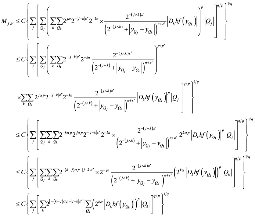
For $q\le p$ , one uses triangular inequality and (34) again to yield

#Math_341# (36)

For $q>p$ , by Hölder’s inequality and (33) again, one obtains

$\begin{array}{c}{M}_{f,V}\le C\{{\displaystyle \underset{j}{\sum }}{\left[{\displaystyle \underset{k}{\sum }{2}^{\left[-\left(k-j\right)\alpha p-\left|j-k\right|{\epsilon }^{″}\right]q/p}}\right]}^{\left(1-p/q\right)q/p}{\times {\displaystyle \underset{k}{\sum }{2}^{\left[-\left(k-j\right)\alpha p-\left|j-k\right|{\epsilon }^{″}\right]}}{\left[{\displaystyle \underset{Q_k}{\sum }{2}^{k\alpha p}}{\left|D_{k}bf\left(y_{Q_k}\right)\right|}^p\left|Q_k\right|\right]}^{q/p}\}}^{1/q}\\ \le C{\left\{{\displaystyle \underset{k}{\sum }}{\left[{\displaystyle \underset{Q_k}{\sum }{2}^{k\alpha p}}{\left|D_{k}bf\left(y_{Q_k}\right)\right|}^p\left|Q_k\right|\right]}^{q/p}\right\}}^{1/q}\end{array}$ (37)

Since $y_{Q_k}$ can be replaced by any point in $Q_k$ , it follows that (35) still holds for $1<q<\infty$ . With a modification for $q=\infty$ , (35) holds and therefore

${\left\{{\displaystyle \underset{k}{\sum }}{\Vert {\displaystyle \underset{Q_k}{\sum }{2}^{k\alpha }}\underset{z\in Q_k}{\sup }\left|E_{k}bf\left(z\right)\right|{\chi }_{Q_k}\Vert }_p^q\right\}}^{1/q}\le C{\left\{{\displaystyle \underset{k}{\sum }}{\Vert {\displaystyle \underset{Q_k}{\sum }{2}^{k\alpha }}\underset{z\in Q_k}{\inf }\left|D_{k}bf\left(z\right)\right|{\chi }_{Q_k}\Vert }_p^q\right\}}^{1/q}$ (38)

for $\alpha \in \left(-\epsilon \mathrm{,}\epsilon \right)$ , $\max \left\{\frac{n}{n+\epsilon },\frac{n}{n+\epsilon +\alpha }\right\}<p<\infty$ and $0<q\le \infty$ .

Conversely, if one interchanges the roles of $S$ and $V$ in the proof above, one immediately has

${\left\{{\displaystyle \underset{k}{\sum }}{\Vert {\displaystyle \underset{Q_k}{\sum }{2}^{k\alpha }\underset{z\in Q_k}{\sup }\left|D_{k}bf\left(z\right)\right|{\chi }_{Q_k}}\Vert }_p^q\right\}}^{1/q}\le C{\left\{{\displaystyle \underset{k}{\sum }}{\Vert {\displaystyle \underset{Q_k}{\sum }{2}^{k\alpha }\underset{z\in Q_k}{\inf }\left|E_{k}bf\left(z\right)\right|{\chi }_{Q_k}}\Vert }_p^q\right\}}^{1/q}$ (39)

Hence

#Math_355# (40)

and therefore the proof of part (a) is finished. The proof of part (b) is the same as the one of part (a).

4. Besov Spaces of Para-Accretive Type

Recall a definition and the duals of Besov sequence spaces ${\stackrel{\dot{}}{b}}_p^{\alpha \mathrm{,}q}$ introduced by Frazier and Jawerth [23] [24] . For $\alpha \in ℝ$ and $0<p,q\le \infty$ , the space ${\stackrel{\dot{}}{b}}_p^{\alpha \mathrm{,}q}$ consists of all sequences $s=\left\{s_Q\right\}$ satisfying

${\Vert s\Vert }_{{\stackrel{\dot{}}{b}}_p^{\alpha ,q}}:=(\begin{array}{ll}{\left({\displaystyle \underset{k\in \mathbb{Z}}{\sum }}{\left\{{\displaystyle \underset{\stackrel{Q}{\mathcal{l}\left(Q\right)=2^{-k}}}{\sum }}{\left({\left|Q\right|}^{-\alpha /n-1/2+1/p}\left|s_Q\right|\right)}^p\right\}}^{q/p}\right)}^{1/q}<\infty \hfill & \text{if}0<p<\infty \hfill \\ {\left({\displaystyle \underset{k\in \mathbb{Z}}{\sum }}{\left\{\underset{\begin{array}{c}Q\\ \mathcal{l}\left(Q\right)=2^{-k}\end{array}}{\sup }{\left|Q\right|}^{-\alpha /n-1/2}\left|s_Q\right|\right\}}^q\right)}^{1/q}<\infty \hfill & \text{if}p=\infty \hfill \end{array}$ (41)

Proposition 4.1. ( [25] [26] ) Let $\alpha \in ℝ$ , $1<p\le \infty$ , $0<q\le \infty$ . Then

${\left({\stackrel{\dot{}}{b}}_p^{\alpha ,q}\right)}^{*}\approx {\stackrel{\dot{}}{b}}_{p^{\prime }}^{-\alpha ,q^{\prime }}$ (42)

with the pairing $\langle s,t\rangle ={\displaystyle {\sum }_Q{s}_Q\overline{t_Q}}$ where $s=\left\{s_Q\right\}\in {\stackrel{\dot{}}{b}}_p^{\alpha ,q}$ and $t=\left\{t_Q\right\}\in {\stackrel{\dot{}}{b}}_p^{\alpha ,q}$ . As usual, when $0<q\le 1$ , $q^{\prime }$ interprets as $+\infty$ .

Next one recalls the definition of almost diagonality and the boundedness of almost diagonal matrices acting on Besov sequence spaces.

Definition 4.2. For $\alpha \in ℝ$ and $0<p,q\le \infty$ , let $J=n/p+\max \left\{0,n-n/p\right\}$ . one says that a matrix $A={\left\{a_{{}_{QP}}\right\}}_{{}_{Q,P}}$ is $\left(\alpha \mathrm{,}p\right)$ almost diagonal, denoted by $A\in a{d}_p^{\alpha }$ , if there exist $\epsilon >0$ and $C>0$ such that, for all dyadic cubes $Q$ and $P$ ,

$\left|a_{{}_{QP}}\right|\le C{\left[\frac{\mathcal{l}\left(Q\right)}{\mathcal{l}\left(P\right)}\right]}^{\alpha }{\left(1+\frac{\left|x_{{}_Q}-x_{{}_P}\right|}{\max \left(\mathcal{l}\left(Q\right),\mathcal{l}\left(P\right)\right)}\right)}^{-J-\epsilon }\min \left({\left[\frac{\mathcal{l}\left(Q\right)}{\mathcal{l}\left(P\right)}\right]}^{\frac{n+\epsilon }{2}},{\left[\frac{\mathcal{l}\left(P\right)}{\mathcal{l}\left(Q\right)}\right]}^{\frac{n+\epsilon }{2}+J-n}\right)$ (43)

Proposition 4.3. ( [27] [28] ) Let $\alpha \in ℝ$ , $0<p,q\le \infty$ . If $A\in a{d}_p^{\alpha }$ , then $A$ is bounded on ${\stackrel{\dot{}}{b}}_p^{\alpha \mathrm{,}q}$ .

Theorem 4.4. Suppose that $S={\left\{S_k\right\}}_{k\in \mathbb{Z}}$ is an approximation to the identity defined in Definition 2.1 and set $D_k=S_k-S_{k-1}$ for $k\in \mathbb{Z}$ . For $\alpha \in \left(-\epsilon \mathrm{,}\epsilon \right)$ , $\max \left\{\frac{n}{n+\epsilon },\frac{n}{n+\alpha +\epsilon }\right\}<p<\infty$ , and $0<q\le \infty$ ,

${\Vert f\Vert }_{{\stackrel{\dot{}}{B}}_{b,p}^{\alpha ,q}\left(S\right)}\approx {\Vert \left\{{\left|Q_k\right|}^{1/2}{D}_{k}bf\left(y_{Q_k}\right)\right\}\Vert }_{{\stackrel{\dot{}}{b}}_p^{\alpha ,q}}$ (44)

In particular, the definition of ${\stackrel{\dot{}}{B}}_{b,p}^{\alpha ,q}\left(S\right)$ is independent of the choice of approximations to the identity.

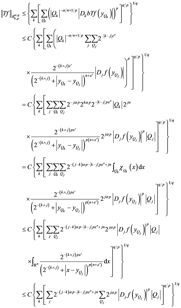
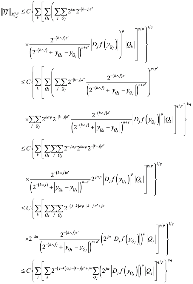
Proof. Let $S={\left\{S_k\right\}}_{k\in \mathbb{Z}}$ and $V={\left\{V_k\right\}}_{k\in \mathbb{Z}}$ be approximations to the identity defined in Definition 2.1. Set $D_k=S_k-S_{k-1}$ and $E_k=V_k-V_{k-1}$ . One wants to show that

#Math_400# (45)

By the Plancherel-Pôlya-type inequality, one has

$\begin{array}{l}{\Vert f\Vert }_{{\stackrel{\dot{}}{B}}_{b,p}^{\alpha ,q}\left(S\right)}={\left\{{\displaystyle \underset{k}{\sum }{2}^{k\alpha q}}{\Vert D_{k}bf\left(x\right)\Vert }_p^q\right\}}^{1/q}={\left\{{\displaystyle \underset{k}{\sum }{2}^{k\alpha q}}{\left({\displaystyle {\int }_{{ℝ}^n}}{\left|D_{k}bf\left(x\right)\right|}^p\text{d}x\right)}^{q/p}\right\}}^{1/q}\\ ={\left\{{\displaystyle \underset{k}{\sum }{2}^{k\alpha q}}{\left({\displaystyle \underset{Q_k}{\sum }}{\displaystyle {\int }_{Q_k}}{\left|D_{k}bf\left(x\right)\right|}^p\text{d}x\right)}^{q/p}\right\}}^{1/q}\\ \le C{\left\{{\displaystyle \underset{k}{\sum }{2}^{k\alpha q}}{\left({\displaystyle \underset{Q_k}{\sum }}{\displaystyle {\int }_{{ℝ}^n}}{\left|D_{k}bf\left(y_{Q_k}\right)\right|}^p{\chi }_{{}_{Q_k}}\left(x\right)\text{d}x)\right)}^{q/p}\right\}}^{1/q}\\ =C{\left\{{\displaystyle \underset{k}{\sum }}{\left[{\displaystyle {\int }_{{ℝ}^n}}{\displaystyle \underset{Q_k}{\sum }}{\left(2^{k\alpha }\left|D_{k}bf\left(x\right)\right|\right)}^p{\chi }_{{}_{Q_k}}\left(x\right)\text{d}x\right]}^{q/p}\right\}}^{1/q}=C{\Vert {\left\{{\left|Q_k\right|}^{1/2}{D}_{k}bf\left(y_{Q_k}\right)\right\}}_{Q_k}\Vert }_{{\stackrel{\dot{}}{b}}_p^{\alpha ,q}}\end{array}$

Apply Proposition 4.3 and the Plancherel-Pôlya-type inequality again to yield

$\begin{array}{c}{\Vert {\left\{{\left|Q_k\right|}^{1/2}{D}_{k}bf\left(y_{Q_k}\right)\right\}}_{Q_k}\Vert }_{{\stackrel{\dot{}}{b}}_p^{\alpha ,q}}\le C{\Vert {\left\{{\left|Q\right|}^{1/2}{E}_{k}bf\left(y_{Q_k}\right)\right\}}_{Q_k}\Vert }_{{\stackrel{\dot{}}{b}}_p^{\alpha ,q}}\\ =C{\left\{{\displaystyle \underset{k}{\sum }}{\left[{\displaystyle {\int }_{{ℝ}^n}}{\displaystyle \underset{Q_k}{\sum }}{\left(2^{k\alpha }\left|E_{k}bf\left(y_{Q_k}\right)\right|\right)}^p{\chi }_{{}_{Q_k}}\left(x\right)\text{d}x\right]}^{q/p}\right\}}^{1/q}\\ \le C{\left\{{\displaystyle \underset{k}{\sum }}{\left[{\displaystyle \underset{Q_k}{\sum }{\displaystyle {\int }_{Q_k}}{2}^{k\alpha p}{\left(\underset{z\in Q_k}{\inf }{E}_{k}bf\left(z\right)\right)}^p{\chi }_{{}_{Q_k}}\left(x\right)\text{d}x}\right]}^{q/p}\right\}}^{1/q}\\ \le C{\left\{{\displaystyle \underset{k}{\sum }}{2}^{k\alpha q}{\left[{\displaystyle \underset{Q_k}{\sum }{\displaystyle {\int }_{Q_k}}{\left|E_{k}bf\left(x\right)\right|}^p\text{d}x}\right]}^{q/p}\right\}}^{1/q}\\ =C{\left\{{\displaystyle \underset{k}{\sum }{2}^{k\alpha q}{\left({\displaystyle {\int }_{{ℝ}^n}}{\left|E_{k}bf\left(x\right)\right|}^p\text{d}x\right)}^{q/p}}\right\}}^{1/q}\\ =C{\Vert f\Vert }_{{\stackrel{\dot{}}{B}}_p^{\alpha ,q}\left(V\right)}\end{array}$

Hence

${\Vert f\Vert }_{{\stackrel{\dot{}}{B}}_{b,p}^{\alpha ,q}\left(S\right)}\le C{\Vert f\Vert }_{{\stackrel{\dot{}}{B}}_p^{\alpha ,q}\left(V\right)}$ (46)

Conversely, if one interexchanges the roles $S$ and $V$ in the proof before, then one has

${\Vert f\Vert }_{{\stackrel{\dot{}}{B}}_{b,p}^{\alpha ,q}\left(V\right)}\le C{\Vert f\Vert }_{{\stackrel{\dot{}}{B}}_p^{\alpha ,q}\left(S\right)}$ (47)

and the proof is completed. $\square$

Form the last theorem, the definition of homogeneous Besov spaces of para-accretive type is independent of the choice of approximations to the identity. For simplicity, one writes ${\stackrel{\dot{}}{B}}_{b\mathrm{,}p}^{\alpha \mathrm{,}q}$ in stead of ${\stackrel{\dot{}}{B}}_{b\mathrm{,}p}^{\alpha \mathrm{,}q}\left(S\right)$ in the sequel.

Theorem 4.5. Suppose $\alpha \in \left(-\epsilon \mathrm{,}\epsilon \right)$ , $\max \left\{\frac{n}{n+\epsilon },\frac{n}{n+\alpha +\epsilon }\right\}<p\le \infty$ and $0<q\le \infty$ .

(a) If $f\in {\stackrel{\dot{}}{B}}_{\mathrm{1,}p}^{\alpha \mathrm{,}q}$ , then $b^{-1}f\in {\stackrel{\dot{}}{B}}_{b\mathrm{,}p}^{\alpha \mathrm{,}q}$ and ${\Vert f\Vert }_{{\stackrel{\dot{}}{B}}_{\mathrm{1,}p}^{\alpha \mathrm{,}q}}\approx {\Vert b^{-1}f\Vert }_{{\stackrel{\dot{}}{B}}_{b\mathrm{,}p}^{\alpha \mathrm{,}q}}$ .

(b) If $f\in {\stackrel{\dot{}}{B}}_{b\mathrm{,}p}^{\alpha \mathrm{,}q}$ , then $bf\in {\stackrel{\dot{}}{B}}_{\mathrm{1,}p}^{\alpha \mathrm{,}q}$ and ${\Vert f\Vert }_{{\stackrel{\dot{}}{B}}_{b\mathrm{,}p}^{\alpha \mathrm{,}q}}\approx {\Vert bf\Vert }_{{\stackrel{\dot{}}{B}}_{\mathrm{1,}p}^{\alpha \mathrm{,}q}}$ .

Furthermore, if $1\le p,q<\infty$ , then the dual space of ${\stackrel{\dot{}}{B}}_{b\mathrm{,}p}^{\alpha \mathrm{,}q}$ is ${\stackrel{\dot{}}{B}}_{\mathrm{1,}{p}^{\prime }}^{-\alpha \mathrm{,}{q}^{\prime }}$ and the dual space of ${\stackrel{\dot{}}{B}}_{\mathrm{1,}p}^{\alpha \mathrm{,}q}$ is ${\stackrel{\dot{}}{B}}_{b\mathrm{,}{p}^{\prime }}^{-\alpha \mathrm{,}{q}^{\prime }}$ .

Proof. If $f\in {\stackrel{\dot{}}{B}}_{\mathrm{1,}p}^{\alpha \mathrm{,}q}$ , by Proposition 2.2,

$f\left(x\right)={\displaystyle \underset{k}{\sum }}{\displaystyle \underset{Q}{\sum }{D}_{k}f\left(y_Q\right)}{\displaystyle {\int }_{Q}b\left(x\right){\mathcal{D}}_k\left(y,x\right)b\left(y\right)\text{d}y}$ (48)

or equivalently,

$b^{-1}\left(x\right)f\left(x\right)={\displaystyle \underset{k}{\sum }}{\displaystyle \underset{Q}{\sum }{D}_{k}b\left(b^{-1}f\right)\left(y_Q\right)}{\displaystyle {\int }_Q{\mathcal{D}}_k\left(y,x\right)b\left(y\right)\text{d}y}$ (49)

By Theorem 4.4, one gets

${\Vert f\Vert }_{{\stackrel{\dot{}}{B}}_{1,p}^{\alpha ,q}}\approx {\Vert \left\{{\left|Q_k\right|}^{1/2}{D}_{k}f\left(y_{Q_k}\right)\right\}\Vert }_{{\stackrel{\dot{}}{b}}_p^{\alpha ,q}}={\Vert \left\{{\left|Q_k\right|}^{1/2}{D}_{k}b\left(b^{-1}f\right)\left(y_{Q_k}\right)\right\}\Vert }_{{\stackrel{\dot{}}{b}}_p^{\alpha ,q}}\approx {\Vert b^{-1}f\Vert }_{{\stackrel{\dot{}}{B}}_{b,p}^{\alpha ,q}}$ (50)

The proof of case (b) is the same. To show the duality. By Propositions 2.2, if $f\in {\stackrel{\dot{}}{B}}_{b\mathrm{,}p}^{\alpha \mathrm{,}q}$ and $g\in {\stackrel{\dot{}}{B}}_{\mathrm{1,}{p}^{\prime }}^{-\alpha \mathrm{,}{q}^{\prime }}$ , then

$f\left(x\right)={\displaystyle \underset{k}{\sum }}{\displaystyle \underset{Q_k}{\sum }{D}_{k}bf\left(y_{{}_{Q_k}}\right)}{\displaystyle {\int }_{Q_k}}{\mathcal{D}}_k\left(y,x\right)b\left(y\right)\text{d}y$ (51)

$g\left(x\right)={\displaystyle \underset{j}{\sum }}{\displaystyle \underset{P_j}{\sum }{D}_{j}g\left(y_{{}_{P_j}}\right)}{\displaystyle {\int }_{P_j}b\left(x\right){\mathcal{D}}_j\left(y,x\right)b\left(y\right)\text{d}y}$ (52)

Thus

$\begin{array}{c}\langle f,g\rangle ={\displaystyle \underset{k}{\sum }}{\displaystyle \underset{Q_k}{\sum }}{\displaystyle \underset{j}{\sum }}{\displaystyle \underset{P_j}{\sum }{D}_{k}bf\left(y_{{}_{Q_k}}\right)D_{j}g\left(y_{{}_{P_j}}\right)}\\ \times \langle {\displaystyle {\int }_{Q_k}}{\mathcal{D}}_k\left(y,x\right)b\left(y\right)\text{d}y,{\displaystyle {\int }_{P_j}b\left(x\right){\mathcal{D}}_j\left(y,x\right)b\left(y\right)\text{d}y}\rangle \end{array}$ (53)

By the estimates for ${\mathcal{D}}_k$ , it is routine to check that the matrix

$\left\{\langle {\displaystyle {\int }_{Q_k}{\mathcal{D}}_k\left(y\mathrm{,}x\right)b\left(y\right)\text{d}y}\mathrm{,}{\displaystyle {\int }_{P_j}b\left(x\right){\mathcal{D}}_j\left(y\mathrm{,}x\right)b\left(y\right)\text{d}y}\rangle \right\}$ (54)

is almost diagonal defined in Proposition 4.3. Thus it is bounded on ${\stackrel{\dot{}}{b}}_{p^{\prime }}^{-\alpha \mathrm{,}{q}^{\prime }}$ , by Proposition 4.1. Thus

$\begin{array}{c}\left|\langle f,g\rangle \right|\le C{\Vert \left\{D_{k}bf\left(y_{{}_{Q_k}}\right)\right\}\Vert }_{{\stackrel{\dot{}}{b}}_p^{\alpha ,q}}{\Vert \left\{D_{j}g\left(y_{{}_{P_j}}\right)\right\}\Vert }_{{\stackrel{\dot{}}{b}}_{p^{\prime }}^{-\alpha ,q^{\prime }}}\\ \le C{\Vert f\Vert }_{{\stackrel{\dot{}}{B}}_{b,p}^{\alpha ,q}}\stackrel{\dot{}}{\Vert }g{\Vert }_{{\stackrel{\dot{}}{B}}_{1,p^{\prime }}^{-\alpha ,q^{\prime }}}\end{array}$ (55)

where the first inequality is followed from Propositions 4.1 and 4.3, and the second inequality is followed from Theorem 4.4. Therefore the duality follows immediately. $\square$

5. An Application

In this section one give a proof of reduced $Tb$ theorem for Besov case.

Proof of Theorem 1.10. For $f\in {\stackrel{\dot{}}{B}}_{\mathrm{1,}p}^{\alpha \mathrm{,}q}$ , by Theorem 4.4, one has

${\Vert Tf\Vert }_{{\stackrel{\dot{}}{B}}_{b,p}^{\alpha ,q}}\le C{\Vert \left\{{\left|Q\right|}^{1/2}{D}_{k}bTf\left(y_{Q_k}\right)\right\}\Vert }_{{\stackrel{\dot{}}{b}}_p^{\alpha ,q}}$ (56)

By the Calderón-reproducing formula,

$\begin{array}{c}{D}_{k}bTf\left(x\right)=D_{k}bT\left({\displaystyle \underset{j}{\sum }}{\displaystyle \underset{Q_j}{\sum }{D}_j}f\left(y_{Q_j}\right){\displaystyle {\int }_{Q_j}}b(\cdot ){\mathcal{D}}_j\left(y,\cdot \right)\left(x\right)b\left(y\right)\text{d}y\right)\\ ={\displaystyle \underset{j}{\sum }}{\displaystyle \underset{Q_j}{\sum }{D}_j}f\left(y_{Q_j}\right){\displaystyle {\int }_{Q_j}}{D}_{k}bTb{\mathcal{D}}_j\left(y,\cdot \right)\left(x\right)b\left(y\right)\text{d}y\end{array}$ (57)

Using the estimate given in [20] Lemma 3.13

$\left|D_{k}bTb{\mathcal{D}}_j\left(y,\cdot \right)\left(x\right)\right|\le C{2}^{-\left|k-j\right|{\epsilon }^{″}}\frac{2^{-\left(k\wedge j\right){\epsilon }^{\prime }}}{{\left(2^{-\left(k\wedge j\right)}+\left|x-y\right|\right)}^{n+{\epsilon }^{\prime }}}$ (58)

implies

$\left|D_{k}bTf\left(y_{Q_k}\right)\right|\le C{\displaystyle \underset{j}{\sum }}{\displaystyle \underset{Q_j}{\sum }{2}^{-\left|k-j\right|{\epsilon }^{″}}}\frac{2^{-\left(k\wedge j\right){\epsilon }^{\prime }}}{{\left(2^{-\left(k\wedge j\right)}+\left|y_{Q_k}-y_{Q_j}\right|\right)}^{n+{\epsilon }^{\prime }}}\left|D_{j}f\left(y_{Q_j}\right)\right|$ (59)

where ${\epsilon }^{\prime }$ and ${\epsilon }^{″}$ are close enough to $\epsilon$ with $0<{\epsilon }^{″}<{\epsilon }^{\prime }<\epsilon$ .

First one considers the case for $p\le 1$ . In this case,

because one mays choose ${\epsilon }^{\prime }$ so that

${\displaystyle {\int }_{{ℝ}^n}}\frac{2^{-\left(k\wedge j\right)p{\epsilon }^{\prime }}}{{\left(2^{-\left(k\wedge j\right)}+\left|x-y_{Q_j}\right|\right)}^{p\left(n+{\epsilon }^{\prime }\right)}}\text{d}x$ (60)

is finite. When $q\le p$ , one uses triangular inequality, and when $q>p$ , one uses Hölder’s inequality to yield

${\Vert Tf\Vert }_{{\stackrel{\dot{}}{B}}_{b,p}^{\alpha ,q}}\le C{\left\{{\displaystyle \underset{j}{\sum }}{\left[{\displaystyle \underset{Q_j}{\sum }}{2}^{j\alpha p}{\left|D_{j}f\left(y_{Q_j}\right)\right|}^p\left|Q_j\right|\right]}^{q/p}\right\}}^{1/q}=C{\Vert f\Vert }_{{\stackrel{\dot{}}{B}}_{1,p}^{\alpha ,q}}$ (61)

so $T$ is bounded from ${\stackrel{\dot{}}{B}}_{\mathrm{1,}p}^{\alpha \mathrm{,}q}$ to ${\stackrel{\dot{}}{B}}_{b\mathrm{,}p}^{\alpha \mathrm{,}q}$ for $p\le 1$ .

Now consider the case $1<p<\infty$ , by Hölder’s inequality

Similarly to this case, when $q\le p$ , one uses triangular inequality, and when $q>p$ , one uses Hölder’s inequality. Thus $T$ extends to a bounded linear operator from ${\stackrel{\dot{}}{B}}_{\mathrm{1,}p}^{\alpha \mathrm{,}q}$ to ${\stackrel{\dot{}}{B}}_{b\mathrm{,}p}^{\alpha \mathrm{,}q}$ . $\square$

It is clear that ${\stackrel{\dot{}}{B}}_{b,p}^{\alpha ,p}={\stackrel{\dot{}}{F}}_{b,p}^{\alpha ,p}$ , and hence ${\Pi }_h^{\left(b\right)}$ is bounded from ${\stackrel{\dot{}}{B}}_{\mathrm{1,}p}^{\mathrm{0,}p}$ to ${\stackrel{\dot{}}{B}}_{b\mathrm{,}p}^{\mathrm{0,}p}$ if $h\in {\stackrel{\dot{}}{F}}_{b\mathrm{,}\infty }^{\mathrm{0,}p}$ by Theorem 1.3 in [8] , where ${\Pi }_h^{\left(b\right)}$ is a paraproduct operator defined by

${\Pi }_h^{\left(b\right)}\left(f\right)\left(x\right)={\displaystyle \underset{k}{\sum }}{\displaystyle \underset{Q_k}{\sum }}{\left|Q_k\right|}^{-1/2}{D}_{k}bh\left(y_{{}_{Q_k}}\right)\langle f,b^{-1}{\Phi }_{{}_{Q_k}}\rangle {\displaystyle {\int }_{Q_k}}{\mathcal{D}}_k\left(z,x\right)b\left(z\right)\text{d}z$ (62)

for some fixed $\Phi \in {\mathcal{D}}_c\left({ℝ}^n\right)$ satisfying ${\displaystyle \int \Phi \left(x\right)\text{d}x}=1$ and $\text{supp}\left(\Phi \right)\subseteq {\left[\mathrm{0,1}\right]}^n$ . It is natural to ask what is the necessary and sufficient condition for the boundedness of paraproduct operators acting from ${\stackrel{\dot{}}{B}}_{\mathrm{1,}p}^{\mathrm{0,}q}$ to ${\stackrel{\dot{}}{B}}_{b,p}^{0,q}$ ?

Supported

Research by author was supported by Ministry of Science and Technology, R.O.C. under Grant #MOST 105-2115-M-259-002.

Conflicts of Interest

The authors declare no conflicts of interest.

References

[1]	Frazier, M. and Jawerth, B., A discrete transform and decomposition of distribution spaces, J. Funct. Anal. 93 (1990), 34-170.
[2]	Frazier, M. and Jawerth, B., Applications of the and wavelet transforms to the theory of function spaces, Wavelets and Their Applications, 377-417, Jones and Bartlett, Boston, MA, 1992.
[3]	Frazier, M., Han, Y.-S., Jawerth, B. and Weiss, G., The theorem for Triebel-Lizorkin spaces, in Harmonic Analysis and Partial Differential Equations (J. Garcia-Cuerva, et al. eds.), Lecture Notes in Math. 1384, Springer, Berlin and New York (1989), 168-181.
[4]	Frazier, M., Torres, R. and Weiss, G., The boundedness of Calderón-Zygmund operators on the spaces Fp α,q , Rev. Mat. Iberoamericana 4 (1988), 41-72.
[5]	Han, Y.-S., Lee, M.-Y. and Lin, C.-C., Hardy Spaces and the Theorem, J. Geom. Anal. 14 (2004), 291-318.
[6]	Han, Y.-S., Lee, M.-Y. and Lin, C.-C., Algebra of Calderón-Zygmund operators associated to para-accretive functions, J. Fourier Anal. Appl. 12 (2006), 581-596.
[7]	Han, Y.-S. and Sawyer, E., Para-accretive functions, the weak boundedness property and the theorem, Rev. Mat. Iberoamericana 6 (1990), 17-41.
[8]	Lin, C.-C. and Wang, K., Triebel-Lizorkin spaces of para-accretive type and a theorem, J. Geom. Anal. 19 (2009), 667-694.
[9]	Lin, C.-C. and Wang, K., Singular integral operators on Trriebel-Lizorkin spaces of para-accretive type, J. Math. Anal. Appl. 364 (2010), 453-462.
[10]	McIntosh, A. and Meyer, Y., Algèbres d’opérateurs définis par intégrales singulières, C. R. Acad. Sci. Paris Sér. I Math. 301 (1985), 395-397.
[11]	Torres, R. (1991) Boundedness Results for Operators with Singular Kernels on Distribution Spaces. Memoirs of the AMS, 442, 1-172. https://doi.org/10.1090/memo/0442
[12]	Wang, K. (1997) The Generalization of Paraproducts and the Full T1 Theorem for Sobolev and Triebel-Lizorkin Spaces. Journal of Mathematical Analysis and Applications, 209, 317-340. https://doi.org/10.1006/jmaa.1997.5381
[13]	Wang, K. (1999) The Full T1 Theorem for Certain Triebel-Lizorkin Spaces. Mathematische Nachrichten, 197, 103-133. https://doi.org/10.1002/mana.19991970108
[14]	David, G. and Journé, J.-L. (1984) A Boundedness Criterion for Generalized Calderón-Zygmund Operators. Annals of Mathematics, 120, 371-397. https://doi.org/10.2307/2006946
[15]	David, G., Journé, J.-L. and Semmes, S. (1985) Opérateurs de Calderón-Zygmund, fonctions para-accrétives et interpolation. Revista Matemática Iberoamericana, 1, 1-56. https://doi.org/10.4171/RMI/17
[16]	Hytonen, T. (2007) Singular Convolution Integrals with Operator-Valued Kernel. Mathematische Zeitschrift, 255, 393-425. https://doi.org/10.1007/s00209-006-0043-x
[17]	Hytonen, T. and Weis, L. (2006) A T1 Theorem for Integral Transformations with Operator-Valued Kernel. Journal für die reine und angewandte Mathematik, 599, 155-200.
[18]	Rubio de Francia, J.L., Ruiz, F.J. and Torrea, J.L. (1986) Calderón-Zygmund Theory for Operator-Valued Kernels. Advances in Mathematics, 62, 7-48.
[19]	Coifman, R.R. and Meyer, Y. (1978) Au-delà des opérateurs pseudo-différentials. Astérisque, Vol. 57, Societe mathematique de France, Paris.
[20]	Han, Y.-S. (1994) Calderóz-Type Reproducing Formula and the Tb Theorem. Rev. Mat. Iberoamericana 10, 51-91. https://doi.org/10.4171/RMI/145
[21]	Deng, D.-G. and Yang, D.-C. (2006) Some New Besov and Triebel-Lizorkin Spaces Associated with Para-Accretive Functions on Spaces of Homogeneous Type. Journal of the Australian Mathematical Society, 80, 229-262. https://doi.org/10.1017/S1446788700013094
[22]	Triebel, H. (1983) Theory of Function Spaces, Monographs in Math. Vol. 78, Birkhauser Verlag, Basel. https://doi.org/10.1007/978-3-0346-0416-1
[23]	Frazier, M. and Jawerth, B. (1985) Decomposition of Besov Spaces. Indiana University Mathematics Journal, 34, 777-799. https://doi.org/10.1512/iumj.1985.34.34041
[24]	Frazier, M., Jawerth, B. and Weiss, G. (1991) Littlewood-Paley Theory and the Study of Function Spaces. CBMS Regional Conference Series, Vol. 79, A.M.S., Providence. https://doi.org/10.1090/cbms/079
[25]	Huang, P.-K. and Wang, K. (2012) Some Operators Acting on Weighted Sequence Spaces and Applications. Taiwanese Journal of Mathematics, 16, 1507-1530.
[26]	Roudenko, S. (2004) Duality of Matrix-Weighted Besov Spaces. Studia Mathematica, 160, 129-156. https://doi.org/10.4064/sm160-2-3
[27]	Huang, P.-K. and Wang, K. (2011) Duals of Weighted Sequence Besov Spaces and Application. Journal of Applied Analysis, 17, 181-205. https://doi.org/10.1515/jaa.2011.012
[28]	Roudenko, S. (2002) Matrix-Weighted Besov Spaces. Transactions of the American Mathematical Society, 355, 273-314. https://doi.org/10.1090/S0002-9947-02-03096-9