RobCoP: A Matlab Package for Robust CoPlot Analysis

Yasemin Kayhan Atilgan¹, Erdinc Levent Atilgan²

¹Department of Statistics, Hacettepe University, Ankara, Turkey.
²Meteksan Defense Ind., Ankara, Turkey.

DOI: 10.4236/ojs.2017.71003                

Abstract

The graphical representation method, Robust CoPlot, is a robust variant of the classical CoPlot method. CoPlot is an adaptation of multidimensional scaling (MDS), and is a practical tool for visual inspection and rich interpretation of multivariate data. CoPlot enables presentation of a multidimensional dataset in a two dimensions, in a manner that relations between both variables and observations to be analyzed together. It has also been used as a supplemental tool to cluster analysis, data envelopment analysis (DEA) and outlier detection methods in the literature. However, this method is very sensitive to outliers. When a multidimensional dataset contains outliers, this can lead to undesirable consequences such as the inaccurate representation of the variables. The motivation is to produce Robust CoPlot that is not unduly affected by outliers. In this study, we have presented a new MATLAB package RobCoP for generating robust graphical representation of a multidimensional dataset. This study serves a useful purpose for researchers studying the implementation of Robust CoPlot method by providing a description of the software package RobCoP; it also offers some limited information on the Robust CoPlot analysis itself. The package presented here has enough flexibility to allow a user to select an MDS type and vector correlation method to produce either classical or Robust CoPlot results.

Keywords

Robust, CoPlot, Multidimensional Scaling, Multivariate Analysis, MATLAB

1. Introduction

CoPlot method, introduced by [1] , is used as a tool for multi-criteria grouping. It consists of two graphs: the first represents the distribution of $p$ dimensional observations over two-dimensional space, whereas the second shows the relation- ships between variables and observations. The main advantage of this method is that it enables the simultaneous investigation of the relations between the observations and between the variables for a set of data. In contrast to many other multivariate methods that produce composites of variables (such as principal component analysis and cluster and factor analysis), CoPlot uses variables that are derived from the original dataset.

Among the wide spectrum of graphical techniques for the treatment of multidimensional dataset, CoPlot method has attracted much attention in recent years in a wide range of areas for various purposes. CoPlot is used for geome- trical representation of multi-criteria decision problems [2] [3] [4] , has been utilized in econometric studies [5] , in energy and environmental modeling [6] , in exploratory data analysis [7] , as an outlier detection tool [8] [9] and for presenting DEA graphically [10] [11] [12] .

Although it is increasingly popular for applications involving multidimen- sional datasets, CoPlot method is sensitive to the outliers. To obtain reliable results, a graphical representation is needed that accounts for the presence of outliers. If the dataset contains outliers, the representation of the variables may deviate strongly from those obtained from the clean data in CoPlot method. Aim of Robust CoPlot method is to reduce impact of outliers and try to fit the bulk of the data [13] .

In this paper, we present the RobCoP package for MATLAB [14] , a software package that implements Robust CoPlot. A first objective in developing this package was to provide researchers with a software package that offers both classical and Robust CoPlot analysis for use with MATLAB; to our knowledge, this is the only package currently providing these features. In the existing literature, there is only one comparable software, which is not open source [15] , enabling only the analysis of classical CoPlot. The package is freely available on the website of the Mathworks file exchange. The site https://www.mathworks.com/matlabcentral/fileexchange/61338-robcop--a-matlab-package-for-robust-coplot-analysis contains the basic functions needed to run the analysis and to obtain the corresponding Robust CoPlot results.

The paper is organized as follows: Section 2 briefly introduces the Robust CoPlot algorithm, and Section 3 gives details about RobCoP written as a set of MATLAB functions. In Section 4, two examples are provided for the application of the package.

2. Methodology of Robust Coplot

2.1. Standardization of Data

The Robust CoPlot method mainly consists of three steps. In order to obtain Robust CoPlot graphs, an MDS embedding of the dataset should be generated. The first step in the algorithm is to obtain standardized data; otherwise, variables measured at different scales do not contribute equally to the analysis [16] . Typical data standardization procedures transform the data to comparable scales by using sample mean and standard deviation. However, these two estimators are very sensitive to outliers, even if only one strong outlier may attract the sample mean and inflate the sample variance. By using median and median absolute deviation (MAD), which are the robust equivalents of these two estimators, possible effects of outliers on the standardization of data are restricted. In Robust CoPlot, the $p$ -dimensional $n$ point data matrix $X_{n\times p}$ is transformed into the standardized matrix $Z_{n\times p}$ in a robust way as follows:

$z_{ij}=\frac{x_{ij}-\text{med}\left(x_j\right)}{\text{MAD}\left(x_j\right)}$ (1)

where $z_{ij}$ is the $i$ -th row and $j$ -th column element of the standardized matrix $Z_{n\times p}$ , $x_j$ is the $j$ -th column of data matrix $X_{n\times p}$ , $\text{med}\left(\mathrm{.}\right)$ is the median function, and $\text{MAD}\left(x_j\right)=1.4826\text{med}\left(\left|x_j-\text{med}\left(x_j\right)\right|\right)$ stands for the median absolute deviation.

2.2. Obtaining MDS Embedding

In the second step, the $p$ -dimensional dataset is mapped onto a two- dimensional space by taking account of the dissimilarity metric obtained from the standardized data matrix. To find a proper embedding of the dataset, metric (classic) or non-metric (ordinary) MDS is used in the literature. Although non-metric MDS (NMDS) can be considered in order to overcome the existence of outliers, Spence and Lewandowsky [17] demonstrated that NMDS may be adversely affected by outliers. The Robust CoPlot method uses the robust MDS (RMDS) proposed by [18] . The main advantage of RMDS is the use of the outlier aware cost function defined as

$f\left(O,Y\right)={\displaystyle \underset{i<j}{\sum }}{\left[{\delta }_{ij}-d_{ij}\left(Y\right)-o_{ij}\right]}^2+\lambda {\displaystyle \underset{i<j}{\sum }}\left|o_{ij}\right|$ (2)

where ${\delta }_{ij}$ is the dissimilarity metric among $i$ -th and $j$ -th row of the standardized matrix $Z_{n\times p}$ , $Y_{n\times 2}$ is the coordinate matrix for two-dimensional space, $d_{ij}\left(Y\right)$ shows the Euclidean distance between $i$ -th and $j$ -th row of coordinate matrix $Y_{n\times 2}$ , $\lambda >0$ is the parameter that controls the assumed number of outliers, and the $i$ -th row $j$ -th column element of the outlier matrix $O$ is $o_{ij}=\mathrm{sgn}\left({\delta }_{ij}-d_{ij}\left(Y\right)\right)\max \left(0,\left|{\delta }_{ij}-d_{ij}\left(Y\right)\right|-\lambda /2\right)$ , which repre- sents the outlier variable.

2.3. Adding Variable Vectors

In the last step of the Robust CoPlot method, vectors representing the variables are located on the obtained robust MDS map. Robust CoPlot decides the direction and magnitude of a vector using the median absolute deviation correlation coefficient (MADCC), ${\rho }_{j,\text{MADCC}}$ , given by [19] .

${\rho }_{j,\text{MADCC}}=\frac{{\text{MAD}}^2\left(u_j\right)-{\text{MAD}}^2\left(k_j\right)}{{\text{MAD}}^2\left(u_j\right)+{\text{MAD}}^2\left(k_j\right)}.$ (3)

Here, $u_j$ and $k_j$ are the robust principal variables given as follows:

$\begin{array}{l}{u}_j=\frac{z_j-\text{med}\left(z_j\right)}{\text{MAD}\left(z_j\right)}+\frac{{\nu }_j-\text{med}\left({\nu }_j\right)}{\text{MAD}\left({\nu }_j\right)}\\ k_j=\frac{z_j-\text{med}\left(z_j\right)}{\text{MAD}\left(z_j\right)}-\frac{{\nu }_j-\text{med}\left({\nu }_j\right)}{\text{MAD}\left({\nu }_j\right)}.\end{array}$ (4)

In (4), $z_j$ stands for the $j$ -th column of standardized data matrix $Z_{n\times p}$ , and ${\nu }_j$ represents the projection values of all $n$ points in the MDS map on the $j$ -th variable vector for a specific direction. For each degree of ${360}^{\circ }$ , the ${\rho }_{j\mathrm{,}\text{MADCC}}$ correlation between the actual values of the variable $j$ and their projection on the vector, ${\nu }_j$ , is calculated. The direction of the vector is determined so that the calculated ${\rho }_{j\mathrm{,}\text{MADCC}}$ value attains maximum.

3. Features of the RobCoP Package

The RobCoP package contains just one main function, RobustCoPlot(), and many auxiliary functions. RobustCoPlot() has one input argument, InStrct, and one output argument, OutStrct. Each argument is a MATLAB structure with different fields. The RobustCoPlot() function can perform NMDS, RMDS analysis with many options for dissimilarity distance function, data stand- ardization type, and MDS initialization method. In addition to MDS analysis, classical and Robust CoPlot analyses can also be performed. The desired analysis is determined by the field values of the input structure, InStrct.

To generate an input structure according to the desired type of analysis, Figure 1 can be used for guidance. The InStrct.X field of the input structure should take the data file name. The data file to be processed by RobCoP should be in comma-separated value (CSV) format. The data columns to be analyzed are selected by using InStrct.DataColNums field. This field should be a one-dimensional matrix whose numeric elements indicate the selected columns from the input CSV file. An optional field, InStrct.ColorColumn, is used for colorizing the data points on the obtained MDS graph. This field should be a scalar that selects the column from the CSV file to be used in colorizing the data points. The InStrct.ColorValues field is a one-dimensional numeric matrix whose elements are the values selected from the column pointed by InStrct. ColorColumn. The RobustCoPlot() can colorize up to six different values selected from InStrct.ColorColumn. In other words, the obtained MDS graph can split the data points by using different shapes and colors up to six groups. The RobustCoPlot() can use three different kinds of distance functions for obtaining the dissimilarity matrix to be used in MDS. The InStrct.DisSimDist field is used for selecting “Euclidean”, “Cityblock”, or “Dominance” distance functions for the analysis. The standardization technique of the dataset can also be chosen by using the InStrct.StdType field. The possible values of the field are “Mean” and “Median”. “Mean” selects the sample mean and sample variance for standardization, while “Median” uses the median value instead of the mean as well as the median absolute deviation (MAD) for variance. The starting point for the MDS analysis is determined by using the InStrct.InitMethod field. The

Figure 1. Formation of input structure InStrct for RobustCoPlot(). (Solid lines indicate required fields, while dashed lines indicate optional ones.).

possible choices are “PCA” for principal component analysis and “Random” for randomly selected starting points. “NMDS” or “RMDS” selection for the MDS analysis is done by using the InStrct.MDSMethod field. If “RMDS” is selected, InStrct.OutlierRatio field should also be defined. The InStrct.OutlierRatio field can take values from $\left(0,1\right)$ interval, and represents the assumed outlier ratio for RMDS analysis. The InStrct.DrawGraph is an optional field which can take values “Shepard”, “MDS”, and “CoPlot”. If this field is not defined, the RobustCoPlot() performs the MDS analysis in silence mode and returns the coordinates of the obtained embedding. “Shepard” option draws the Shepard Diagram only, “MDS” draws the MDS graph, and the “CoPlot” option performs CoPlot analysis. To see all of the graphs, the “ALL” value should be used. If the “CoPlot” option is selected for the InStrct.DrawGraph, the vector correlation method for CoPlot should also be selected by using the InStrct.VecCorrMethod field. If “PCC” is selected the representation of vectors is implemented by the Pearson correlation coefficient; if “MADCC” is selected, representation is implemented by the median absolute deviation correlation coefficient.

The fields of the output structure, OutStrct, vary by the MDS analysis type selected. The following two fields, OutStrct.StressValue and OutStrct.Embedding, are the returned fields regardless of the MDS method selected. The OutStrct. StressValue field returns the Kruskall stress value of the obtained resultant MDS embedding. The Kruskall stress value shows the quality of the obtained two-dimensional mapping of the multivariate data, and a smaller value means good representation. The OutStrct.Embedding field returns the coordinates of the data points found by the selected MDS method. If “RMDS” is selected as the InStrct.MDSMethod, then OutStrct contains an additional field, OutStrct.Outlier, containing non-zero elements showing the distances that are deemed as outliers during the RMDS analysis.

4. Illustrative Examples

Robust CoPlot method considers all the variables as well as the observations simultaneously to obtain two dimensional map. Correlations among the va- riables, relations among the observations and mutual relationship among the observations and their measuring variables can be seen by a single graphical representation. Besides possible outliers which are located far from the bulk of the data can easily been detected.

In this section, we present and illustrate the use of the RobCoP package on the dataset frequently used in the DEA analysis to show the economic performance of China’s cities [20] . Step-by-step instructions will be given on how to obtain classic and Robust CoPlot maps. In the dataset, there are six variables for 35 of China’s cities (Decision Making Units/DMU): labor (ILF), working fund (WF), investment (INV), gross industrial output value (GIOV), profit and taxes (P&T), and retail sales (RS). All of the examples given in this section use the same dataset to make comparisons between classical and Robust CoPlots. The first two examples are related to the embedding of the observations into two- dimensions and the following two examples are prepared for CoPlot results.

The RobustCoPlot() function takes the CSV file as an input dataset. The first line of the input data file should contain the names of the variables, and the number of columns in the file should be equal to the number of variable names. In other words, the input file should not contain any unnamed columns. The first few lines of the CSV file used in the examples are given in Table 1 for

Table 1. First a few lines of the input CSV file.

reference. After adding the package to MATLAB path, the following code is used for importing the input data file.

Then, ChineseCities.csv, which has 36 rows representing the name of variables and observations and 8 columns representing the variables and color values, is ready for the analysis.

4.1. NMDS and RMDS Analysis

The RobCoP package supports non-metric MDS analysis, which is used in classic CoPlot analysis, and RMDS, which is used in Robust CoPlot analysis. The first column of ChineseCities.csv file is excluded from the analysis because it contains the observation number. The last column, COLOR, is generated for coloring the resultant MDS embedding in which the numbers are given in a way to sort the profit and taxes (P&T) values at the sixth column of the dataset. The color value assignment is performed according to the defined ranges in Table 2. The color column is also omitted from the analysis.

In order to allow comparisons among variables on different scales, RobCoP package standardizes the data. In this example to generate non-metric MDS embedding, “Mean” is selected for standardization type.

The MDS embedding of the dataset requires a set of distances between the observations. Although given example uses city-block distance, various distance metrics can be selected to create distance matrix in the RobCoP package.

For the starting point of the MDS embedding, “PCA” (Torgerson) is selected by using the InStrct.InitMethod field.

To produce non-metric MDS results, following code snippet can be used. To obtain NMDS map, InStrct.DrawGraph field is selected as “MDS”. Similarly, to

obtain Shepard diagram, it is entered as “Shepard”.

After preparing the input structure, a single command is required to perform analysis.

For the given example, the obtained non-metric MDS embedding of the dataset is shown in Figure 2. The Shepard diagram of the non-metric MDS analysis is shown in Figure 3. The Shepard diagram is a scatter plot of the distances between points in the MDS plot against the observed proximities, and ideally the actual proximities versus the predicted proximities fall on a straight line. If the Shepard diagram resembles a step-wise or stair-case function, a degenerate solution may be obtained. The points on the Figure 4 adhere cleanly to a straight line.

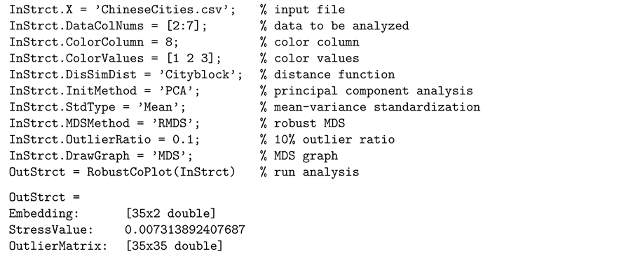
The following code snippet can be used for robust MDS analysis of the same dataset. Only the InStrct.MDSMethod field of the input structure is changed to a

Table 2. Color value assignment table according to P&T(6) variable.

Figure 2. Obtained embedding for non-metric MDS analysis of ChineseCities.csv file.

Figure 3. Obtained shepard diagram for non-metric MDS analysis of ChineseCities.csv file.

Figure 4. Obtained shepard diagram for robust MDS analysis of ChineseCities.csv file.

“RMDS” value, and since robust MDS is selected, the InStrct.OutlierRatio value should be given. The outlier ratio for the example is assumed to be 10% [13] . In addition, the output structure also contains an OutStrct.OutlierMatrix field to show which distances are taken as outliers during RMDS analysis. The obtained results are shown in Figure 5 and Figure 4. Although Figure 2 and Figure 5 seem similar for the given example, as the percentage of outliers in the data

Figure 5. Obtained embedding for robust MDS analysis of ChineseCities.csv file.

increases contamination of the predicted proximities in NMDS solution in- creases.

4.2. Robust CoPlot Analysis

The maps generated so far are the NMDS and RMDS maps without variables. In this section, a second map, superimposed on the first, consisting of vectors for each variable is generated. The following code snippet provides classical CoPlot analysis. The user needs to know that the data matrix standardization type and computation method of the vector correlation coefficients, InStrct.VecCorr- Method, should be chosen as “Mean” and “PCC” respectively to obtain classical analysis results (see Figure 6).

The following code snippet enables to draw Robust CoPlot. The data matrix standardization type and the computation method of the vector correlation coefficients have to be specified as “Median” and “MADCC” to obtain robust analysis results (see Figure 7).

5. Conclusion

In this paper, we present the RobCoP package for performing graphical display method of multivariate data in MATLAB. Our main objective while developing this package was to provide a useful tool for helping the researchers to depict the multivariate data in the presence of outliers. This paper makes an important

Figure 6. Classical CoPlot analysis of ChineseCities.csv file.

Figure 7. Robust CoPlot analysis of ChineseCities.csv file.

contribution by presenting a new software package that supplies the reader Robust CoPlot analysis as well as robust MDS and classical CoPlot analysis with open source code. Until recently there was no package for robust version of CoPlot analysis and robust MDS. The package presented in this paper addresses these issues. We believe that this package will be used in various areas, especially in applied statistics.

Conflicts of Interest

The authors declare no conflicts of interest.

References

[1]	Lipshitz, G. and Raveh, A. (1994) Application of the Co-Plot Method in the Study of Socio-Economic Differences between Cities: A Basis for a Differential Development Policy. Urban Studies, 31, 123-135. https://doi.org/10.1080/00420989420080071
[2]	Raveh, A. (2000) Co-Plot: A Graphic Display Method for Geometrical Representations of {MCDM}. European Journal of Operational Research, 125, 670-678. https://doi.org/10.1016/S0377-2217(99)00276-3
[3]	Cangur, S., Ercan, I. and Ozkaya, G. (2015) Co-Plot Method: A Research on Tobacco Control in the European Region. Epidemiology, Biostatistics and Public Health, 12, e11480-1–e11480-9.
[4]	Shoval, N. and Raveh, A. (2004) Categorization of Tourist Attractions and the Modeling of Tourist Cities: Based on the Co-Plot Method of Multivariate Analysis. Tourism Management, 25, 741-750. https://doi.org/10.1016/j.tourman.2003.09.005
[5]	Raveh, A. (2000) The Greek Banking System: Reanalysis of Performance. European Journal of Operational Research, 120, 525-534. https://doi.org/10.1016/S0377-2217(98)00384-1
[6]	Demirhan, H. and Atilgan, Y.K. (2015) New Horizontal Global Solar Radiation Estimation Models for Turkey Based on Robust Coplot Supported Genetic Programming Technique. Energy Conversion and Management, 106, 1013-1023. https://doi.org/10.1016/j.enconman.2015.10.038
[7]	Lipshitz, G. and Raveh, A. (1998) Socio-Economic Differences among Localities: A New Method of Multivariate Analysis. Regional Studies, 32, 747-757. https://doi.org/10.1080/00343409850119436
[8]	Mahlberg, B. and Raveh, A. (2012) Co-Plot: A Useful Tool to Detect Outliers in Dea. Social Science Research Network.
[9]	Bravata, D.M., Shojania, K.G., Olkin, I. and Raveh, A. (2008) Coplot: A Tool for Visualizing Multivariate Data in Medicine. Statistics in Medicine, 27, 2234-2247. https://doi.org/10.1080/00343409850119436
[10]	Huang, H. and Liao, W. (2012) A Co-Plot-Based Efficiency Measurement to Commercial Banks. Journal of Software, 7, 2247-2251.
[11]	Adler, N. and Raveh, A. (2008) Presenting DEA Graphically. Omega, 36, 715-729. https://doi.org/10.1016/j.omega.2006.02.006
[12]	Nath, P., Mukherjee, A. and Pal, M.N. (2001) Identification of Linkage between Strategic Group and Performance of Indian Commercial Banks: A Combined Approach Using DEA and Co-Plot. International Journal of Digital Accounting Research, 1, 125-152. https://doi.org/10.4192/1577-8517-v1_7
[13]	Atilgan, Y.K. (2016) Robust Co-Plot Analysis. Communications in Statistics—Simulation and Computation, 45, 1763-1775. https://doi.org/10.1080/03610918.2013.875571
[14]	The MathWorks Inc. (2016) MATLAB—The Language of Technical Computing, Version 2016a. The MathWorks Inc., Natick.
[15]	Talby, D. (2015) The Visual Co-Plot, Version 5.5.
[16]	Borg, I. and Groenen, P.J. (2005) Modern Multidimensional Scaling: Theory and Applications. Springer Science & Business Media, Berlin.
[17]	Spence, I. and Lewandowsky, S. (1989) Robust Multidimensional Scaling. Psychometrika, 54, 501-513. https://doi.org/10.1007/BF02294632
[18]	Forero, P. and Giannakis, G. (2012) Sparsity-Exploiting Robust Multidimensional Scaling. IEEE Transactions on Signal Processing, 60, 4118-4134. https://doi.org/10.1109/TSP.2012.2197617
[19]	Shevlyakov, G. and Smirnov, P. (2011) Robust Estimation of the Correlation Coefficient: An Attempt of Survey. Austrian Journal of Statistics, 40, 147-156.
[20]	Charnes, A., Cooper, W.W. and Li, S. (1989) Using Data Envelopment Analysis to Evaluate Efficiency in the Economic Performance of Chinese Cities. Socio-Economic Planning Sciences, 23, 325-344. https://doi.org/10.1016/0038-0121(89)90001-3