Inverse Source Locating Method Based on Graphical Analysis of Dye Plume Images in a Turbulent Flow ()
1. Introduction
A problem commonly encountered in emergent chemical leakage is the quick localization of the leaking source using the data observed at monitoring sites. If the source location of pollutant material is identified based on the observation data through some possible ways, the remediation and risk assessment can be carried out accordingly. However, the inverse source localization is difficult in most cases, as almost all flows related with material dispersion in nature are turbulent. In turbulent flow, the material dispersion is a result of a wide spectrum of eddy motions, with the large-scale motions behaving like a spatially in-homogeneous mean flow and producing coherent meandering of a pollutant plume, while the small-scale motions diffusing the material and mixing it with the ambient medium [1] . When a material is released into turbulent flow, it may cover numerous possible routes before being sensed by measurement downstream. This complexity challenges the inverse estimation of the source location, which, instead of an inverse deterministic problem, is a probability problem, that is to say, due to the chaotic feature and irreversibility of turbulent flow, the exact location of material source cannot be determined. What people can obtain is the region where the source possibly locates in, with corresponding possibility or confidence. However, in any case, having a deep investigation of the dispersion process and the scalar field of material dispersion is essential.
There have been many studies about the material dispersion in turbulent flow. Taylor [1] concerned the problem of dye released continuously into a turbulent flow from a single point source, and focused on how far on average the fluid particles migrate from the source after a certain time. Different mechanisms of diffusion, i.e., relative diffusion or meandering diffusion, dominate the material dispersion according to whether the time after release is larger than the integral time scale or otherwise. Similar aspects were proposed by Richardson a few years after Taylor’s diffusion theory, regarding the relative separation of two fluid particles released into a turbulent flow. From Richardson’s diffusion theory [1] , the question of how fast the dye plume enlarges was discussed. Besides Taylor’s and Richardson’s turbulent diffusion theories, several approaches aimed to predict the mean concentration field were also proposed by many researches [2] [3] . Considering the inadequate information mean concentration contains in case of pollutant risk assessment, concentration fluctuation was investigated quantitatively [4] [5] [6] [7] and the peak to mean ratio was also predicted [6] . In order to describe the intermittency characteristics of scalar field in turbulent flow, the intermittency was defined and studied [8] [9] [10] . Based on those previous researches [8] - [16] , many quantities are found to be related with the diffusion distance of dye plumes: these quantities includes time-average concentration, plume width, concentration fluctuation quantities, intermittency, concentration burst quantities, spatial correlation, and integral length. Some inverse estimation methods for source localization have been proposed based on these diffusion-distance-related quantities [16] [17] .
Recently, instead of on the plume, there are researches focusing on the possible information contained in the high-intensity pulses or spikes of the scalar field, which can be used for the inverse estimation of source location [18] [19] [20] [21] . Endo et al. [18] extracted high concentration pulses through pattern recognition and binarization. The characteristic of concentration pulses embedded in the plume was investigated and the diffusion width of the pulses was found to be proportional to the streamwise distance from the source. In reference [19] , the mean pulse height, pulse onset slope, and probability of pulse height were concerned, and it was indicated that these features might be used as directional cues for source localization. The time-averaged value of the rise slope was also found to vary systematically with the distance from the source [20] . Page et al. [21] declared that the high-intensity spike encounters dominate the tracking motion of a crab, and high frequency of odorant spike encounters terminates its upstream movement.
These high-intensity pulses are called dye patches in this paper, which contain much information about source location. The starting point of this study is to extract the characteristic of dye patches which is a function of the streamwise distance from the release source. Experiments were conducted to the dye solution dispersion process released into a fully-developed turbulent water flow in a channel. Instantaneous concentration fields of dye plumes are recorded using a planar laser-induced fluorescence (PLIF) technique. The release is isokinetic and continuous and we set seven observation sites downstream of the release point designed to see the dependence of dye-patch characteristics on the streamwise distance from the source. The image recorded is two- dimensional, while it is assumed that the spanwise location of the point source is known, and the source localization problem in this paper is simplified to be a one- dimensional problem. Such an assumption, although too ideal and rarely practical, is necessary for the preliminary study and exploration of a possible source location estimation method. After experimental measurement by PLIF technique, the dye dispersion images were processed by graphical analysis method following three steps: binarization, labeling, and pixel counting. Statistical analysis was performed concerning the dye patch distribution characteristics, based on which, the dependence of those characteristics on the streamwise distance from the source was discussed. A possible source- locating estimation method would be proposed in this study.
2. Experiment Setup
Figure 1 shows the experiment apparatus of flow loop and the measurement section with PLIF technique. The streamwise distance between the dye release point and the downstream observation site is called “diffusion distance” in this paper, denoted by dx, as shown in Figure 1(b), and the diffusion distance normalized by half channel height δ is . This study concerns the dye patch characteristics of the dye plume and its relationship with the streamwise distance from the release point. Seven observation sites (diffusion distances) are selected:
  = 10, 25, 30, 35, 40, 45, and 60. The section where the observation sites locate is called “measurement section”, which is well designed for optics access. Rhodamine WT is used as the dye, and the injection from the nozzle is isokinetic with local flow. The dispersion images of Rhodamine WT are captured by PLIF technique. Both in Figure 1(a) and Figure 1(b), the coordinate system
![]()
Figure 1. Schematic diagram of experiment apparatus. Figure 1(b) shares the same coordinate system and unit with Figure 1(a). (a) Experiment setup. (b) PLIF measurement setup.
defines x as the streamwise direction, y as the wall-normal direction and z for the spanwise direction with the coordinate origin located at the nozzle tip. The measurement section is 1000 mm in length and starts 2000 mm downstream the inlet of a transparent channel flume. The flume is 4300 mm long with a rectangular cross section of 20 mm (2δ) in height (y direction) by 250 mm in width (z direction). At the inlet of the flume, a honeycomb rectifier is installed to straighten the flow. The distance the flow covers between the inlet of the flume and the measurement section is long enough to assume the flow there is fully developed. A high-speed camera is fixed below the flume, and laser is used to illuminate the center plane of the channel, which is aligned with the dye-source nozzle height. The optical cutoff filter is placed over the camera lens to only pass the fluorescence to the camera sensor. A time-synchronization equipment (not shown in the figure) is used to synchronize the pulse laser with the high speed camera. The fluid tem- perature is kept at 25˚C, and the Reynolds number Re (Re = 2δUb/ν) is 20,000, with Ub being the bulk velocity of the channel flow and ν being the kinematic viscosity of water.
The images obtained by the PLIF technique in this experiment are two-dimensional (on the central x-z plane). The number of images for each observation site is 500, providing many plume-shape samples at 500 time instants for each .
.
3. Graphical Analysis
Firstly, from raw dye-plume images obtained by PLIF, the background noise was removed: some examples of the images are shown in Figures 2(a1)-(a5). Note that all the images in Figure 2 share the same coordinate system and length scale, as shown in Figure 2(a1). Figure 2(a1) and Figure 2(a2) are the dye plume images for  = 10 at two different instants, while Figures 2(a3)-(a5) are the dye plume images for the other three sampled
 . Each shown image represents the dye plume shape at one among the corresponding 500 instants of each observation site. Due to highly fluctuating motions of turbulence, the passive dye distribution is also fluctuating and chaotic. The dye plume image at one instant is absolutely different from the other instants, but we expected some common features underlying among them. For such complex phenomena, from instantaneous dye distributions, only qualitative features can be inferred: both spatial and temporal concentration distributions are fluctuating and intermittent with high concentration areas that distribute randomly in one snapshot, while totally changed in terms of shape, location, and the total number at other snapshots. To have a deeper analysis, the results must be statistical ones.
This research focuses on the statistical characteristics of these high concentration areas (“dye patches” below). Dye patches are defined as the areas above a certain concentration level. Beforehand, three-step graphical analysis is used to extract all the dye patches from the PLIF images with their respective areas and perimeters. The three steps are binarization, connected components labeling, and pixel counting.
3.1. Binarization to Highlight Dye Patches
Figures 2(b1)-(b5) are the corresponding binarized images of Figures 2(a1)-(a5). It can be seen, dye patches are highlighted against the background. This binarization is based on Otsu’s method [22] to remove low concentration and noise based on automatically determined threshold. The reason of carrying out binarization based on the threshold by the automatic threshold determining method instead of the threshold given artificially is mainly to avoid the subjective definition of dye patches.
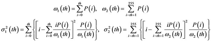
Otsu’s method assumes that the image contains two classes of pixels following bi-modal histogram (e.g., foreground and background pixels) and then calculates the optimum threshold separating those two classes so that their combined spread (intra- class variance: the variance within the class) is minimal. The intra-class variance is
![]()
![]()
Figure 2. Examples of PLIF obtained images and binarized images: (a1)-(a5) are the dye plume images obtained by PLIF measurement, and (b1)-(b5) are the corresponding binarized images of (a1)-(a5) based on Otsu’s method.
defined as,
 (1)
(1)
where 1 and 2 denote the two classes separated by the threshold th (here, 1 is the part under threshold th; while 2 is the class over th); ω1(th) and ω2(th) are the probabilities of the two classes;  and
and  are the variances of the two classes; they are calculated by
 (2)
(2)
where P(i) is the probability of the pixel with gray level being i (0 ≤ i ≤ 255).
By Otsu’s method, the optimum threshold th is obtained by exhaustively searching for the threshold value that minimizes the intra-class variance.
Based on the determined threshold for each PLIF image, the PLIF image is binarized, like Figures 2(b1)-(b5) show. Compared with the original images, the binarized images are much clearer to recognize dye patches as the contour of the patches are high- lighted. At far downstream, there are connected large dye patches, while many spot- like dye patches can be seen near the source (small ). Besides, it is seen that the dye patches distribute randomly with neither direction preference nor stretching tendency towards one direction. The result reflects that the shear stress by the mean flow velocity gradient can be neglected and the assumption of a homogeneous turbulent flow in the channel central region is reasonable.
3.2. Connected Components Labeling to Separate Dye Patches Apart
Based on the above-obtained binarized images, high-intensity dye patches are isolated and extracted by connected components labeling [23] . This labeling scans an image and groups its pixels into components based on pixel connectivity, i.e., all pixels in a connected component are in some way (this paper concerns 8-neighbor connectivity) connected and these pixels are assigned as the same intensity. Once all groups have been determined, each pixel is labeled with a gray level according to the component it belongs to. Figure 3 shows an example of connected components labeling, the highlighted areas on the bi-level image [shown in (a)] is labeled into different gray levels according to the connectivity [shown in (b)]. After labeling, the area of one gray level denotes an independent high-intensity dye patch. However, it should be noted that the different gray levels on the image after labeling have no relationship with the intensity or concentration value in this patch, and we use different gray levels just for visualization here.
3.3. Pixel-Counting to Calculate Areas and Perimeters of Dye Patches
Each independent dye patch is consisted of an integer number of pixels and at least covers one pixel. The area of each independent dye patch S is calculated by counting the pixels it covers. As for the perimeter LP of each dye patch, it is calculated by the edge of the labeled dye patch. The obtained areas and perimeters are normalized, respectively, by δ2 and δ, and denoted as S* and .
.
4. Dye Patch Characteristics Related with Diffusion Distance
4.1. Fractal Dimension
Considering that the diffused patches are irregular and fragmented in shape, like clouds, mountains, trees and coastlines, dye patches are seen as fractals in this research, and fractal dimension is defined to describe the shape irregularity of a pattern [24] [25] , which, unlike the topological dimension, is a non-integer number.
Mimicking the topological dimension that S1/2 µ L, for a dye patch of perimeter LP and area S, we can have the relationship of normalized LP and S as
 (3)
(3)
![]()
Figure 3. Example of post processing of labeling individual dye patches. In (b), different levels of gray color indicate different dye patches.
with the fractal dimension Df of dye patch, reflecting its fractal geometry or irregularity. By application of logarithm operation on the both sides, Equation (3) transforms to,
 (4)
(4)
Equation (4) demonstrates that Df can be determined directly from the distribution of  by linear regression. Figure 4 shows the relationship of
 ![]() of the dye patches in binarized images in logarithmic relationship, and the profiles for three diffusion distances are given. From Figure 4, the dots concentrating around a linear relationship between
of the dye patches in binarized images in logarithmic relationship, and the profiles for three diffusion distances are given. From Figure 4, the dots concentrating around a linear relationship between ![]() and
and ![]() is observed. According to Equation (4), from the slope of the dots marked line, the fractal dimension Df can be calculated, and Figure 5 shows the averaged fractal dimension Df by 500 images against the diffusion distance
is observed. According to Equation (4), from the slope of the dots marked line, the fractal dimension Df can be calculated, and Figure 5 shows the averaged fractal dimension Df by 500 images against the diffusion distance![]() .
.
In Figure 5, for images taken at different observation sites, the dye patches extracted have a fractal dimension of around 1.35 in the two-dimensional view, independent of the diffusion distance. In fractal view, it is induced that the dye patches obtained through our graphical analysis procedures are self-similar [26] . The irregularity of the dye patches, no matter the patches are small or large, are the same.
4.2. Dye Patch Area Distribution
To investigate the distribution of individual dye patch areas S for each diffusion distance, the probability distribution function (PDF) is employed here. Equation (5) gives the way to calculate PDF of logS* for each![]() .
.
![]()
Figure 5. Variation of fractal dimension Df of dye patches at seven diffusion distance![]() .
.
![]() (5)
(5)
For logS* which is within the interval of [a, b], its probability density is the ratio of the number of dye patches with logS* within [a, b] among the entire total. Figure 6 shows the PDF curves for some of the sampling diffusion distances, with the dots referring to the probability of the corresponding statistical interval and the error bars denoting the standard deviation in each statistical interval. The dots for one ![]() are fitted by one spline.
are fitted by one spline.
Based on Figure 6, we may make some discussions. According to the literature, e.g., [1] , eddies in turbulent flow are scaled over a wide range. For turbulent dispersion, which is directly affected by the turbulent motion and is the combined result of advection by mean flow, relative diffusion by small-scale eddies, meandering diffusion by large-scale eddies, and molecular diffusion at the Bachelor scale [1] , the dye patch area distribution seems reasonable. Normalized dye patch areas cover a wide range of scales from 10−4 to 10. For different observation sites, the results are similar in shape, with a single maximum peak of the PDF curve. Through quantitative analysis, the following three points can be concluded:
1) The dye patch areas with largest appearance probability are in Kolmogorov scale.
From Figure 6, it is found that the maximum probability of logS* tends to remain around −3.5 for the diffusion distances designed, that is S* ≈ 10−3.5 or
![]() (6)
(6)
Based on bulk Reynolds number, the friction Reynolds number is calculated [27] ,
![]() (7)
(7)
![]()
Figure 6. Probability density function of logS* at different diffusion distance ![]() from source.
from source.
The friction Reynolds number can be expressed by the friction velocity uτ as
![]() (8)
(8)
Combining Equations (6), (7) and (8) leads to
![]() (9)
(9)
Now let us turn to the Kolmogorov scale. Tsukahara et al. [28] gave the specific values of the Kolmogorov scale at the channel center for two Reτ of 180 and 395: the Kolmogorov length scale η is, respectively, 3.7ν/uτ and 4.6ν/uτ. It can be inferred that, for the present Reτ = 576, most of the high-concentration fluorescent dye patches resulted from turbulent diffusion are in the Kolmogorov scale. As the Kolmogorov scale describes the smallest scale of turbulence below which the viscosity dominates, this phenomenon can reflect the effect of turbulent mixing and stirring by eddies.
For the scalar field, the Bachelor scale describes the smallest length scales of fluctuations in scalar concentration that can exist before being dominated by molecular diffusion. The Bachelor scale in this research is smaller than the Kolmogorov scale, since the Schmidt number is high. From Figure 6, it can be inferred that the diffusion of concentration is less effective than diffusion of vorticity, which is reasonable for the water flow [1] . Besides, as ![]() increases, an obvious shift of the peak location towards small logS* is observed, which reflects the accumulation of stirring and mixing effect into the Kolmogorov scale as the dye patches move downstream.
increases, an obvious shift of the peak location towards small logS* is observed, which reflects the accumulation of stirring and mixing effect into the Kolmogorov scale as the dye patches move downstream.
2) Towards downstream, scales of large and small dye patches tend to separate.
For far downstream locations, dye patches with large area exist, while for near-source regions, the dye patches tend to be spot-like with small areas. This is because that, near the source, the concentration field is more fluctuating both in space and in time. By binarization, the relatively high concentration spots are highlighted, while the relatively low concentration surroundings are depressed in the binarized image. While for far downstream regions, the dye spreads widely due to relative diffusion and the concentration field is more homogeneous than near the source. By binarization, the regions with small spatial concentration variation are deemed as one connected region, the binarized dye patches tend to have lager areas. Meanwhile, as mentioned above, the stirring and mixing effect of turbulence tends to produce more dye patches of Kolmogorov scale, and the lower bound of the area is limited by the measurement resolution of the experiment. By combination of the two aspects, the two scales of larger patches and smaller patches tend to separate towards downstream.
3) Towards downstream, the kurtosis of logS* increases.
Figure 7 shows the kurtosis of the probability density distribution of logS* for each![]() . As from Figure 6, it is seen that when
. As from Figure 6, it is seen that when ![]() increases, an obvious sharpened probability density distribution of logS* is seen, although for
increases, an obvious sharpened probability density distribution of logS* is seen, although for ![]() and 30 the change is not obvious. This aspect may be quantified by the kurtosis (or the flatness factor) Ku of logS*. In probability theory and statistics, the kurtosis is a measure of whether the distribution of data is peaked or flat compared with a normal distribution. Distribution with high kurtosis tends to have a distinct peak near the mean and vice versa. The sharpened profile of the PDF curve corresponds to an increase of Ku. Quantitatively, the kurtosis is calculated as the ratio of the fourth moment and the second moment squared [29] . For data set
and 30 the change is not obvious. This aspect may be quantified by the kurtosis (or the flatness factor) Ku of logS*. In probability theory and statistics, the kurtosis is a measure of whether the distribution of data is peaked or flat compared with a normal distribution. Distribution with high kurtosis tends to have a distinct peak near the mean and vice versa. The sharpened profile of the PDF curve corresponds to an increase of Ku. Quantitatively, the kurtosis is calculated as the ratio of the fourth moment and the second moment squared [29] . For data set ![]() with mean value rmean, Ku is calculated by
with mean value rmean, Ku is calculated by
![]() (10)
(10)
![]()
Figure 7. Variation of kurtosis of PDF as a function of diffusion distance![]() .
.
In Figure 7, the solid square represents the average and the error bar shows the standard deviation. Assume the appearance of the deviation at ![]() and 45 from the main trend is acceptable, we may confirm that, as mentioned above, Ku increases with an increasing
and 45 from the main trend is acceptable, we may confirm that, as mentioned above, Ku increases with an increasing![]() . It means that the distribution of the appearance probability of dye patches with different areas become more peaked when the plume spreads downstream, that is dye patches with certain areas (near the Kolmogorov scale) dominate at farther downstream.
. It means that the distribution of the appearance probability of dye patches with different areas become more peaked when the plume spreads downstream, that is dye patches with certain areas (near the Kolmogorov scale) dominate at farther downstream.
5. Proposal of a Source Locating Method by Kurtosis
For simplicity and reliability, we expect a linear approximation of the relationship between Ku and![]() . The linear regression is used to quantify the strength of the relationship between Ku and
. The linear regression is used to quantify the strength of the relationship between Ku and![]() . With the least square fitting method, we have the following model,
. With the least square fitting method, we have the following model,
![]() (11)
(11)
Due to the turbulent characteristics, Equation (11) is never the only expression between Ku and![]() . As the inverse problem of dye-source estimation of in the turbulent flow is rather a probability problem, where the estimated source location always involves some uncertainty. The reliability of Equation (11) is evaluated, as shown in Figure 8 and Figure 9.
. As the inverse problem of dye-source estimation of in the turbulent flow is rather a probability problem, where the estimated source location always involves some uncertainty. The reliability of Equation (11) is evaluated, as shown in Figure 8 and Figure 9.
In Figure 8, ER is the uncertainty in the inverse estimation of the source location, calculated by,
![]() (12)
(12)
In Equation (12), ![]() is the estimated normalized distance from the point source to the observation site by the inverse estimation, and
is the estimated normalized distance from the point source to the observation site by the inverse estimation, and ![]() is the true value of the
is the true value of the
![]()
Figure 8. Relative errors of source location estimated by Equation (11) from different number of available images Nimage, as a function of![]() .
.
![]()
Figure 9. Inverse estimation accuracy evaluation by benefit over cost based on Equation (13).
normalized distance between the point source and the observation site.
In Figure 9, B/C means a benefit-cost ratio, which reflects the benefit obtained per PLIF image. The value of B/C is defined as
![]() (13)
(13)
where Nimage is the number of PLIF images used for the inverse estimation. For simplicity, the average uncertainty instead of the standard deviation is considered here.
In Figure 8, two ![]() regions are marked, one is near the source around
regions are marked, one is near the source around![]() , while the other is from
, while the other is from ![]() to 60. As is seen, uncertainties exist when using Equation (11) to inversely estimate the source location. Considering the irreversibility of turbulent dispersion, the uncertainties are reasonable. Generally speaking, the inverse estimation for
to 60. As is seen, uncertainties exist when using Equation (11) to inversely estimate the source location. Considering the irreversibility of turbulent dispersion, the uncertainties are reasonable. Generally speaking, the inverse estimation for ![]() with more images produces more accurate results; however, such superiority is only obvious for the estimation based on observation at
with more images produces more accurate results; however, such superiority is only obvious for the estimation based on observation at ![]() downstream. However, in general, the inverse estimation based on observation at
downstream. However, in general, the inverse estimation based on observation at ![]() has very large uncertainties, even as large as 180% when using 10 images, and nearly 120% when using 50 images. Just as Briggs [30] mentioned, Gaussian plume models are not applicable for the near-source region, because near the source concentration approaches infinity. Similarly, the proposed method are not well applicable for the near- source regions either, because near the source the dye plume approaches unity and the dye patch distribution is in an extreme case. While for estimation based on observation at
has very large uncertainties, even as large as 180% when using 10 images, and nearly 120% when using 50 images. Just as Briggs [30] mentioned, Gaussian plume models are not applicable for the near-source region, because near the source concentration approaches infinity. Similarly, the proposed method are not well applicable for the near- source regions either, because near the source the dye plume approaches unity and the dye patch distribution is in an extreme case. While for estimation based on observation at ![]() or farther, the relative error of the inverse estimation drops a lot compared with the uncertainty at
or farther, the relative error of the inverse estimation drops a lot compared with the uncertainty at![]() , with most of the uncertainty located within ±40% range. Due to the limit of the experiment, we can only speculate that, if the uncertainty of ±40% is acceptable, the inverse estimation based on observation from
, with most of the uncertainty located within ±40% range. Due to the limit of the experiment, we can only speculate that, if the uncertainty of ±40% is acceptable, the inverse estimation based on observation from ![]() to (at least) 60 is accurate and feasible.
to (at least) 60 is accurate and feasible.
Figure 9 reveals that, through increasing the number of PLIF images, the accuracy is not proportionally improved. Combined with the result in Figure 8, it is inferred that when observed at proper locations, the inverse estimation of the source location based on the dye patch characteristics is feasible even when using very limited number of images. It is understood that the dye patches even on one PLIF image contain rich information reflecting the diffusion distance, which allows us to conduct the source localization based on limited PLIF images. This method provides a promising way to locate the source location inversely from limited available information by directly taking graphical analysis of the PLIF obtained plume images.
The above is the introduction and evaluation of a possible source-locating method for dye released into a turbulent flow. Figure 10 gives a schematic conclusion of the proposal of this method. The left part is the inverse problem to be solved. The right part in the gray box is the model proposal. Then the inverse problem can be solved by applying the obtained model. From the model proposal to its application, the flow condition must be the same. That is to say, the model serves the source estimation problem where it comes.
6. Conclusions
This study proposes a possible inverse estimation method for the source location of a dye (or pollutant: passive scalar) plume in a turbulent flow. A water-channel experiment was carried out simulating the dispersion process of injected dye solution into a quasi-homogeneous turbulence in the channel central region, and the dye plume images
![]()
Figure 10. Flow chart of inverse estimation of source location based on the kurtosis of the PDF of logarithm dye patch areas. The right part (in the box) is the model proposal, the left part (out of the box) is the application of the model for inverse estimation of the source location.
are captured through a PLIF technique. To investigate the variations of plume characteristics as a function of the diffusion distance from the source, seven downstream observation sites were selected for taking the PLIF images. Through graphical analysis of binarization, connected components labeling, and pixel-counting, dye patches in the plume images are extracted with the areas and perimeters quantitatively known.
The dye patch area distributions are analyzed quantitatively and that with maximum occurrence probability is found to be of the Kolmogorov scale, verifying the effect of turbulent eddies on the scalar diffusion. Besides, towards downstream, clear separation in scale of the large dye patches and small dye patches is observed, which is due to the mixing effect and relative diffusion. To see the diffusion-distance dependence, the fractal dimension of the extracted dye patches is calculated and found to be almost constant. While, the kurtosis of the logarithm dimensionless dye patch area is found to be a function of the diffusion distance from the source. Based on the relationship between the kurtosis and the diffusion distance, a possible inverse source-locating method is proposed. From the evaluation result of the uncertainty of this method, considering that the source localization of a turbulent dispersion can never be deterministic as the turbulent flow is irreversible, the uncertainty of the inverse estimation is reasonable and the estimation accuracy of this method is more acceptable when the PLIF images are taken at a proper distance from the source. Moreover, the proposed method is able to conduct the source localization based on limited number of PLIF images, which is due to the large number of dye patches contained even in one PLIF image. As turbulent dispersion is complex, the present method would provide a promising way for inverse- problem solving. To reduce the uncertainty and to realize a quick problem solving based on limited data are still important in future works.