Multi-Dimension Support Vector Machine Based Crowd Detection and Localisation Framework for Varying Video Sequences ()
1. Introduction
Tracking is defined as the process of finding the most similar object appearance. The objective of crowd tracking is to determine the states of the desired object in a video sequence. Tracking of moving objects in crowds and motion based detection are important features in many applications such as surveillance system, recognizing the activity of object, human machine interface, monitoring of traffic, motion capture, safety purpose, medical systems and robotics. To determine the location and/or shape of the object in every frame, tracking is used in higher-level applications. An appearance model can be used to depict the desired target in visual tracking. There are three models available for tracking the particular object namely motion model, appearance model and update model. The perfect examples of motion model are Kalman filter and particle filter which are used to depict the probable states of an object. Although many models have been developed, still object tracking seems to be a challenging problem due to the rapid and random changes in the appearance of the object due to abrupt motion in crowd, pose variation, occlusion, varying viewpoints and varying lighting conditions (illumination), compared to all other factors.
Numerous schemes have been proposed for object tracking. The object can be represented in several manners, for example: points [1] , articulated models [2] , contours [3] , or optical flow [4] . In our paper, we have chosen motion and geometric structure based representation of the objects, which can be determined between successive frames. Some of the approaches use model-based techniques which usually assume a priori shape model of a human body represented by stick figures [5] [6] or 2-D contours [7] or volumetric shapes. The appearance-dependent technique uses low-level features to represent the target motion. The motion analysis is based on statistical investigation of these features and/or simple heuristics. The initial frame [8] [9] based static appearance models are used in many object tracking process. But these methods are not capable to cope up with important appearance changes. A key issue in object analysis is finding efficient descriptors for object appearance. Different traditional methods such as Linear Discriminant Analysis (LDA) [10] , Supervised Principle Component Analysis and the recent 2D PCA [11] have been studied. The gray-scale invariance is the most important feature for video sequences that have uneven illumination or great variability. Randen and Husoy [12] concluded that the degree of computational complexity of the texture measures is too high in their research. It involves dozens of different spatial filtering methods. For future research the development of powerful texture measures can be extracted and can be done with a low-computational complexity. Several examples of generative tracking techniques are Eigen tracking [13] , WSL tracking [14] and IVT [15] . The object model is frequently updated online in order to adapt to appearance changes as in [15] . The appearance variations are highly non-linear and hence multiple subspaces [16] and non-linear manifold learning methods [17] have been introduced. Apart from category-based methods, exemplar-based methods treat positive samples particularly to avoid the visual-incoherence problem. Chum and Zisserman [18] have developed the exemplar-based classification model to empirically represent object categories. In [19] [20] local distance function learning method by employing triplets, and the focal image which represents the exemplar has been proposed.
Traditional template based tracking algorithms can be divided in two categories. They are offline and online tracking method. In offline method, an object model is either learned offline (by using similar visual examples) or learned by using the first few frames. In both the cases once the object model is generated, immediately a predefined metric model is used to determine the position in adjacent frames. Illustration of this type of tracking algorithms includes Kernel based methods [21] and appearance models [22] . The subspace-based appearance models use the matrices of the pixel values in the image regions that are flattened into vectors and the overall statistical information of every pixel used for finding the vectors is found through PCA. Black and Jepson [23] present a subspace learning-based tracking algorithm. More reliable and accurate schemes like extended dynamic programming [24] are still complex to be employed in problems having maximum number of observations and objects. In spite of several research analyses, detection of crowded objects in many complex situations is still a very good research area [3] [4] .
For developing an efficient tracking algorithm, appearance and update model research is concentrated recently. Appearance model can be further divided into discriminative and generative model. The generative model focuses on the knowledge about the object to develop the appearance model whereas the discriminative model simultaneously considers both the knowledge about the background and object. As object tracking can be considered as binary classification task which can be done by extract- ing the object from its background. The discriminative appearance model is most suitable for the successful implementation of object tracking. Collaborative models are most acceptable for tracking the finer details of the object which are based on above models.
In order to obtain a clear-cut idea about the collaborative model, multi-view learning method has been proposed in this paper. The proposed paper uses collaborative model which is a combination of different sub-models with each having different properties. The collaborative model can be framed by combining two discriminative models or a generative and a discriminative model. In this paper, the first step is to consider three different features namely gray scale value (GSV), histogram of oriented gradients (HOG) and local binary pattern (LBP). Gabor features and gray level co-occurrence matrix (GLCM) are to represent the unique properties of objects from various perspectives. The gray scale feature which can be obtained by vectoring the image regions, gives the basic description of the object image. The histogram of oriented gradients indicates the edge information and gradient statistic features. HOG feature can also be widely applied in object detection task.
The local binary pattern is used to describe the texture of the object. This can also be used to improve the accuracy in object recognition. These features can be further classified into five complementary views of feature subspaces originally. As these features have different attributes, it inspires us to select them as the multiple views of features. All these features are robust to noise and occlusions since they have structural and local attributes. For further combinations, the sub-models are made by using support vector machines dependent learners. The second step is to determine the weight of each learner. SVM learner gets the confidence score in every frame while tracking the crowd. Each learner’s weight has been calculated through the confidence score that is obtained from probability distribution function. To estimate the ambiguity of probability distribution, entropy can be used. Thus entropy can be taken as the measure of weights. The multi view SVMs are combined based on the entropy criterion by a combination strategy that is proposed in this paper. The state-of-the-art techniques are used to estimate the weights depending on the previous performances of the learners whereas the entropy criterion estimates the weights by the current performance of the learners. The flow of the paper next is as follows. Section 2 reviews the literature survey. In Section 3 our proposed algorithm is presented in detail. Experimental results computed using MATLAB software are analysed in Section 4 and conclusion part is included in Section 5.
2. Proposed Methodology
In our proposed paper we intend to build more accurate and robust SVM based detection system. Here we propose a method using fast algorithm for crowd tracking and detection that learns crowd activities and behavior, which finds application in clearing the vehicle traffic during peak hours. To develop crowd detection system that aids fast rescue of lives in times of crises like accident, bomb blast, natural calamities are the motivation behind the research this work. To construct a more comprehensive appearance model using additional feature-Grayscale, Histogram of Oriented Gradients, Local Binary Pattern, Gabor features and Gray Level Co-occurrence Matrix (GLCM) is the major innovation presented in our paper. So that accuracy and robust nature of SVM based crowd detection system is improved. We also present an entropy strategy for the collaboration which determines the weights according to the current performance of each classifier attempting to make a more accurate combination. Finally, we employ FAST (Features from Accelerated Segment Test) algorithm in crowd detection for local features extraction. The block diagram of proposed method is presented in Figure 1.
Here, we have combined two algorithms for crowd detection and localization. They are SVM (Support Vector Machine) and FAST (Features from Accelerated Segment Test) algorithms. In this new approach first the input video sequence is converted into 25 to 29 frames per second. Then the frame is segmented to separate the foreground from the background to eliminate the not required area of study in that image. This can
![]()
Figure 1. Block diagram of proposed methodology.
be done by using a clustering process called Adaptive mean shift algorithm. The adaptive mean shift (AMS) algorithm is an advanced version of mean shift algorithm. This method is utilized because it converges quickly. After segmentation the crowd or a particular target can be detected and localized using a hybrid algorithm that combines both SVM and FAST algorithm.
2.1. Adaptive Mean-Shift Iterative Segmentation Algorithm Units
It is a non-parametric iterative algorithm. This algorithm is applicable for lot of purposes like finding modes, clustering etc. In our paper we use this algorithm to do segmentation by means of adaptive mean shift iterative process. The feature space is considered as probability density function in adaptive mean shift. The input is considered to be sampled from the probability density function when it is a set of points. The clusters or dense regions are considered as the mode of probability density function when it is present in the feature space. Mean shift is also used to identify the clusters associated with the given mode. Mean shift associates each data point with the nearby peak of the probability density function of the datasets. Mean shift then defines a window around each data point and computes the mean of the data point using the window. The center of the window is shifted to the mean and until it converges the algorithm is repeated. The window shifts to deeper region of the dataset after each iteration.
The algorithm works as follows:
1) A window is fixed around each data point.
2) The mean of data is computed within the window.
3) Then the window is shifted to the mean and the steps are repeated till convergence.
2.1.1. Kernels
A kernel is a function which obeys the following preliminaries,
 , where
 . (1)
. (1)
Some examples of kernels include:
1) Rectangular
 . (2)
. (2)
2) Gaussian
 . (3)
. (3)
3) Epanechnikov
 . (4)
. (4)
2.1.2. Kernel Density Estimation and Gradient Ascent Nature of Mean Shift
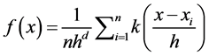
The non-parametric way to calculate the density function of a random variable is by using Kernel density estimation. This is called as the Parzen window technique. Given a kernel K, bandwidth parameter h, Kernel density estimator for a given set of d-dimen- sional points is as follows
 . (5)
. (5)
Mean shift is considered to be based on Gradient ascent on the density contour. The generic formula for gradient ascent is,
 . (6)
. (6)
Applying it to the kernel density estimator we get,
 (7)
(7)
 . (8)
. (8)
Setting it d to 0 we get,
 . (9)
. (9)
Finally,
 . (10)
2.1.3. Iterative Mean Shift and Proof of Convergence
The Mean shift considers the points of the feature space as a probability density function. Dense regions in feature space are mapped to local maxima or modes. So, the gradient ascent is performed for each data point on the local estimated density until it convergence. The stationary points obtained via gradient ascent indicate the modes of the density function. All the points associated with the same stationary point belong to the same cluster.
Assuming,
 . (11)
We have
 . (12)
The quantity m(x) is called as the mean shift. So mean shift procedure can be summarized as that for each point , Compute mean shift vector
  and move the density estimation window by
 , and repeat the process till convergence. Using a Gaussian kernel as an example,
 (13)
(13)
![]() . (14)
. (14)
Using the kernel profile, we have to prove that![]() , Using the Equation (14) we can write the above equation as,
, Using the Equation (14) we can write the above equation as,
![]() . (15)
. (15)
Thus we have proven that the sequence ![]() is convergent.
is convergent.
2.2. Learning and Training of Multi-View SVMs
We have introduced object tracking based on multi-view SVM (MVS) algorithm. This algorithm is implemented as follows. The MVS tracker which uses different views of features (gray level value, HOG, LBP, Gabor feature, GLCM) are implemented in the particle filter structure. The gathered multi-view SVMs are used for representing the object and implementing the appearance model. Then the entropy strategy is used for combining the multi-view SVMs and is built into the particle filter structure in order to obtain the results of tracking. The subspace evolution strategy is also used in this algorithm for updating, adjusting update rate and also for providing guidance to retrain multi-view SVMs in online. The construction of tracking method is actually based on the discriminative model. However the discriminative model formulates the tracking as a binary classification problem. For accurate object representation, the multi-view features based SVMs are trained to implement a collaborative appearance model. The fusion strategy is used for building up this collaborative model.
Figure 2 shows how to construct an appearance model. From an image, samples are prepared from positives and negatives samples of the image. The positive samples and the negative samples are selected around the objects. The five features named gray level, HOG, LBP, Gabor features and GLCM are obtained from these samples and they are sent to the respective SVMs to perform training. Let the positive samples be Ap and the negative samples be An. The selection would be better if the samples are selected from the cropped image regions. By distance based rule, for example, for mi, its label is defined as![]() . It is also represented in pairs as {mi, ni}. Let k(m0) and k(mi) be the location of target and sample to be trained, respectively. By distance based rule,
. It is also represented in pairs as {mi, ni}. Let k(m0) and k(mi) be the location of target and sample to be trained, respectively. By distance based rule,
Case (1):![]() , mi is a positive sample. (16)
, mi is a positive sample. (16)
Case (2):![]() , mi is a negative sample (17)
, mi is a negative sample (17)
where d1, d2 and d3 are predefined thresholds
We take d1 = 2 pixels,
![]() , and
, and ![]() (18)
(18)
where w and h are width and height of the pixels respectively. Practically it is not necessary to select the target region in the video sequence because the training samples are automatically selected in this method. This rule is also updating the training samples in frames. From samples the features are extracted to represent the objects. The gray scale features is obtained by dividing the 2D image region and it gives the basic
![]()
Figure 2. Object tracking based on Multi-View SVM with five different features for detection.
description of the object. The HOG feature has powerful detection capability and it is based on gradient of the image. The LBP feature is used for representing texture of the image. It also has recognition capability. Gabor feature is used for edge detection, texture description and discrimination. The purpose of using gray level co-occurrence matrix is to examine the texture of the object based on spatial relationship between the pixels. The features that are extracted are denoted as ygray, yHOG, yLBP, ygaber, ygaber and yGLCM, respectively. For example the pair of feature vectors is represented as![]() . The cropped image is normalized for convenience. These pairs of features are trained into the SVM classifier to build appearance model. The results are obtained with classification problem for which the SVM will use a separate plan done by maximizing the positive and negative image margins. Assume (k) Î {gray, HOG, LBP, GLCM, Gabor} and i Î {+1, −1}. The optimization problem is represented by,
. The cropped image is normalized for convenience. These pairs of features are trained into the SVM classifier to build appearance model. The results are obtained with classification problem for which the SVM will use a separate plan done by maximizing the positive and negative image margins. Assume (k) Î {gray, HOG, LBP, GLCM, Gabor} and i Î {+1, −1}. The optimization problem is represented by,
![]() . (19)
. (19)
Its subjected condition is:
![]() (20)
(20)
where, Ck trade-parameter and ![]() slack variable. Due to independency between the features, the sub-problem can be expressed as,
slack variable. Due to independency between the features, the sub-problem can be expressed as,
![]() , k Î {gray, HOG, LBP, GLCM, Gabor}. (21)
, k Î {gray, HOG, LBP, GLCM, Gabor}. (21)
The dual problem of lagrangian multiplier algorithm is:
![]() . (22)
. (22)
Figure 3 explains about training SVMs in particle filter and using entropy criterion to determine the final confidence score. Equation (22) is subjected to,
![]() (23)
(23)
where ![]() are Lagrange’s multipliers. By solving these problems the multiple views of learners represents the appearance model of the object. For a sample m, the confidence score is calculated as,
are Lagrange’s multipliers. By solving these problems the multiple views of learners represents the appearance model of the object. For a sample m, the confidence score is calculated as,
![]() . (24)
. (24)
The final confidence score is:
![]() , k Î {gray, HOG, LBP, GLCM, Gabor} (25)
, k Î {gray, HOG, LBP, GLCM, Gabor} (25)
![]() is the weighted parameter of each SVM features.
is the weighted parameter of each SVM features.
2.3. Entropy Computation
The particles represent possible state of the object and simulate the state distribution. Hence, the confidence score of each particle is required for the tracking result. The two steps of particle parameters are:
![]()
Figure 3. Block diagram of particle filter.
1) Prediction step:
![]() . (26)
. (26)
2) Update step:
![]() (27)
(27)
where ![]() are observation variables.
are observation variables.
The observation model is denoted by ![]() and the transition model is represented as
and the transition model is represented as![]() .
.
![]() , where S is called as state space and px, py is translation in x and y direction, where tx, ty is scale variation in x and y direction.
, where S is called as state space and px, py is translation in x and y direction, where tx, ty is scale variation in x and y direction.
Consider N number of particle for approximating the state space. The changes in video sequences must be small and random. These particles must obey multi-dimen- sional Gaussian distribution. Examples: LI and IVT tracking method (same assumptions are taken). Each particle represents candidate sample. Confidence score are calculated over these samples. We normalize the candidate samples mi (![]() ) to extract all the features and calculate corresponding confidence score. Thus the final confidence score is obtained. However combination is a key problem which can be overcome by considering horizontal and vertical translation. In different sequences the final confidence score which shows that different features of different abilities. The scores of particles by min-max rule in the range (0, 1) is,
) to extract all the features and calculate corresponding confidence score. Thus the final confidence score is obtained. However combination is a key problem which can be overcome by considering horizontal and vertical translation. In different sequences the final confidence score which shows that different features of different abilities. The scores of particles by min-max rule in the range (0, 1) is,
![]() . (28)
. (28)
Then the scaled confidence score is:
![]() (29)
(29)
where
![]() . (30)
. (30)
The entropy of the confidence scale distribution is,
![]() . (31)
. (31)
This is determined after calculating entropy of each distribution. The likelihood function is,
![]() (32)
(32)
where ![]() is the similarity weighted parameter which is used for re-sampling.
is the similarity weighted parameter which is used for re-sampling.
By Maximum A Posteriori rule,
![]() (33)
(33)
where Xopt is the optimal candidate sample and its corresponding optimal state Sopt is determined.
2.4. Subspace Evolution Used in Update Model
As the background and object often changes during video sequencing, an online update strategy named subspace evolution strategy is used. This controls the updating process in video sequencing. This method involves constructing subspace to the object and evolving it in accordance with the change of the object. It involves two stages, finding the distance between the subspace and optimal sample in the current frame and retraining strategy. We can use the positive and negative samples to span subspace of the object and we construct the new optimal sample Xopt based on l1 minimization. The training sample set is![]() , solving the problem by LARS algorithm
, solving the problem by LARS algorithm
![]() (34)
(34)
where ![]() _ reconstruction coefficient vector,
_ reconstruction coefficient vector, ![]() are l1 and l2 norms.
are l1 and l2 norms.
![]() is the regularization parameter (0.01). The reconstruction error for positive samples is,
is the regularization parameter (0.01). The reconstruction error for positive samples is,
![]() . (35)
. (35)
This error indicates distance between Xopt and subspace of the appearance and decides to whether update or not as per the following cases.
Case (1): If err < Th (threshold), then Xopt is represented by existing subspace.
Case (2): If err > Th, then the change of appearance exceeds the representation subspace capacity and hence it has to b evolved. This avoids the occlusion samples and thus posse’s robust nature.
2.5. Improved Fast Algorithm for Crowd Detection
There are several feature detectors that are really good, but they are not fast enough. One of the best examples is SLAM (Simultaneous Localization and Mapping) mobile robot in which computational resources are limited. As a solution to this problem, FAST (Features from Accelerated Segment Test) algorithm have been proposed. Here, A pixel P is selected in the image that is to be considered as a required point or not. Let its intensity be![]() . the appropriate threshold value t is selected. A circle of 16 pixels is considered around the pixel under test as shown in Figure 4. (See the image below)
. the appropriate threshold value t is selected. A circle of 16 pixels is considered around the pixel under test as shown in Figure 4. (See the image below)
There are 16 pixels chosen from the selected object and from here the corner pixel p is chosen between the pixels ![]() (maximum brighter value) and
(maximum brighter value) and ![]() (maximum darker value). To exclude a large number of non-corners, a high-speed test was proposed. This test analysis is done only on the four pixels at 1, 9, 5 and 13. Suppose P is the corner pixel then there should be 3 pixels between
(maximum darker value). To exclude a large number of non-corners, a high-speed test was proposed. This test analysis is done only on the four pixels at 1, 9, 5 and 13. Suppose P is the corner pixel then there should be 3 pixels between ![]() and
and![]() , otherwise P can never be a corner. The full segment test criterion can then be applied to the successful
, otherwise P can never be a corner. The full segment test criterion can then be applied to the successful
![]()
Figure 4. Selection of a correct threshold value from the object using fast algorithm.
candidates by analyzing all pixels in the circle. This detector shows high performance but there are several drawbacks which are lesser optimal performance because its performances are related to the distribution of corner appearances. Multiple features are estimated for the points adjacent to one another. So we are going to machine learning a Corner Detector using improved Fast algorithm. Here we have considered a set of images for training. The algorithm is performed in every image to calculate feature points. The 16 pixels are stored around every feature point as a vector. To get feature vector P, this has to be done for all the images. Each pixel (say x) in these 16 pixels can have one of the following three states:
![]() (36)
(36)
The feature vector P is further divided into 3 subsets, ![]() depending on the above states. A new Boolean variable is defined as
depending on the above states. A new Boolean variable is defined as ![]() which is true if P is a corner and false otherwise. By using the ID3 algorithm (decision tree classifier) to examine each subset using the variable
which is true if P is a corner and false otherwise. By using the ID3 algorithm (decision tree classifier) to examine each subset using the variable ![]() to get the knowledge about the true class. It leads to the selection of the x value which gives the basic information about whether the candidate pixel is a corner of the crowd to be detected, which is measured from the entropy of
to get the knowledge about the true class. It leads to the selection of the x value which gives the basic information about whether the candidate pixel is a corner of the crowd to be detected, which is measured from the entropy of![]() . When the entropy becomes 0, the above process must be stopped and the final resultant frame can be used for fast detection in other images.
. When the entropy becomes 0, the above process must be stopped and the final resultant frame can be used for fast detection in other images.
3. Experimental Result
In our method, we executed and tested the performance using 8 public challenging video sequences. Firstly, to analyze the performance of our method, we experimented the different sequences with our algorithm under critical conditions. We compare our method with the other state-of-the-art tracking methods and also compared with similar methods. Secondly, we measure the performance of different combinations of the various features in our method. Later, we study the role of the subspace evolution update model and the entropy criterion. Our tracking method is initialized as follows. The first step is to normalize the size of the image region is kept as 30 × 30, for feature extraction. Both the number of positive and negative samples are set to 50. A 5-pixel widow size and 9 orientations are assigned to the HOG descriptor [25] . A 10-pixel window is used for the LBP descriptor [26] . The dimensions of feature vectors are designated as 900, 324, 105, 245 and 522 respectively. It is assumed that both the model complexity and the training errors of each SVM have equivalent mask. The value is mathematically set to 1, where k ϵ {gray, HOG, LBP, GLCM, Gabor}. The number of the particles in the particle filter is set to 300, where the individual particle depicts the trimmed image region of fixed size 30 × 30. A value of 0.5 is set to the similarity weight, and a value of 0.005 is assigned to the threshold. In all the experiments conducted by us, these parameters are fixed. The 8 video sequences are obtained from different scenes and they also include critical conditions such as pose variations, illumination changes, occlusions, scale variations, clutter background, etc. The complete information of the dif- ferent video sequences including the sizes and the frame numbers is given in Table 1.
We have a detailed comparison with several different tracking methods, including Frag [27] , IVT [28] , MIL [29] , OAB [30] , L1 [31] , VTS [32] , TLD [33] , MTT [34] , CT [35] , VTD [36] , Struck [37] and PartT [38] . All these trackers apply different representation or inference models. The codes of these trackers are all available in public and we can alter the parameters attentively so that better performance results can be obtained. By analyzing the result of our SVM method both quantitatively and qualitatively, we consider two complementary evaluation parameters for the quantitative analysis. They are, centre location error (CLE), tracking success rate (TSR). By averaging the pixel errors between the obtained centers of tracking results and the ground truth, we can calculate the centre location error. The location error is directly proportional to the centre location error value. i.e., smaller the CLE value, smaller the location error. The reduced value of CLE for our algorithm is shown in Figure 5.
![]()
Table 1. Sizes and frame numbers of testing sequences.
![]()
Figure 5. Comparison results of the average center location errors of competing trackers (in pixels).
The best performance of our proposed algorithm through TSR value is shown in Figure 6. Tracking is successful only if the score and TSR gives the ratio of the number of the successful frames and the total. The failure rate (FR) is the third performance parameter, which can be explained as the number of times the tracking is failed in the total video sequence. In our tracking process, to continue the tracking, the tracker will be reinitialized at the failure frame depending on the ground truth and the failure times will be added 1, if and only if the score in current frame. The failure times, which represents the reinitialization times, for the entire video sequences tracking process is set to the value 0.1. The robustness of the trackers can be estimated from the FR value as it is based on the entire sequences. Based on the results obtained from our experiment on different video sequences we can infer that the proposed method performs better in terms of average CLE value as depicted in Table 2 and average TSR value as shown in Table 3. We also observed that the location error is smoother and lower on our input sequences. For most of the sequences our tracking algorithm is able to track the object
![]()
Figure 6. Comparison results of the tracking successful rates of competing trackers.
![]()
Table 2. Comparison results of the average center location errors of competing trackers (in pixels).
![]()
Table 3. Comparison results of the tracking successful rates of competing trackers.
successfully. From Figure 7 we can analyze the performance of our tracker in qualitative manner. To deal with occlusion, fast motions, illumination changes, scale variations, complex background and pose variations, our system uses local features.
Example of a human video with crowded objects chosen as below to show the greater performance of our algorithm in detail with multiview SVM features and Improved FAST algorithm.
Figure 7 first shows gray scale feature of the obtained input that is the frame of video represents the crowded objects, second it also represents the local binary pattern of the video frame considered for our analysis.
Figure 8 and Figure 9 represent the HOG and GABOR features that are extracted from the input frame. Figure 10 and Figure 11 calculate the moving pixels obtained by comparing the current frame and the reference frame.
And Figure 12 shows the modified expectation maximization algorithm output. Figure 13 shows the confidence score distribution of the input frame obtained by using SVM classifier.
Figure 14 shows the object tracking output obtained using SVM algorithm and Figure 15 shows the crowd density determination based on crowd movement obtained by using FAST algorithm.
The update model can be used in our method to reduce the effect of occlusions. The IVT method does not perform well on sequences with sudden illumination changes. But our algorithm can overcome this limitation as we use features that are robust to illumination changes. We can deal scale with variation existing in the video sequences by integrating the approaches based on MTP, VTD and VTS. When the object moves fast or having sudden movement, the performance of our method exceeds to that of remaining methods. The SVM proposed in our paper employs discriminative models and various combination strategies so that it can be robust against complex background. Since our method uses suitable on-line learning strategy and collaborative model we
![]()
Figure 7. Extracting features from the input frame.
can successfully track the changes in human’s gesture. It is difficult to studying the changes in appearance during tracking for accurate representation. The classification accuracy for rapid appearance changes of the tracked target, cannot reflect the performance of the classifier on current frame, it leads to inaccuracy in the calculation of weights. The sparce collaborative is the model that is been used commonly for these kind of situations in the current scenario. The disadvantages of the stated methods are it cannot be adaptable to different conditions, as it empirically fixes the weight of each model in advance. For learning the appearance online, we present a novel subspace evolution strategy that controls the update rate adaptively. Potential applications of MVS tracking method is multi-media information processing, since the object of interest often needs to be tracked with the preprocessing stage. MVS can also provide a coarse segmentation for editing operations. Additionally MVS can also track each part of the object of interest in pixel domain. The challenge lies on his method further will be removing of full occlusions and dealing with drastic rotations of the object.
4. Conclusion
In this paper, we present a novel MVS tracking method with multiple views of SVMs. The FAST algorithm is used to detect the CROWD. This method follows multi-view learning framework and integrates five views of features. Each view of the features represents a special characteristic of the object and the combination leads to a more comprehensive representation of the appearance. In this paper, we present a novel MVS tracking method with multiple views of SVMs. This method follows multi-view learning framework and integrates three views of features. Each view of the features repre- sents a special characteristic of the object and the combination leads to a more comprehensive representation of the appearance. Furthermore we propose a novel entropy criterion to determine the weights of the multi-view SVMs which make the collaboration more accurate and robust. Besides, we also propose a novel subspace evolution strategy combining with the retraining method to complete the model update. The experimental results demonstrate that our MVS tracking method has the comparable per- formance with some state-of-the-art methods under various challenging conditions such as avoiding occlusions when objects under movement and illumination changes due to varying environmental conditions. Moreover, the MVS can be considered as a framework in which other views of features with more expressive power can also be embedded in to the hardware such as system on chip (SOC) and can improve the speed and performance in the future.