A Back Propagation-Type Neural Network Architecture for Solving the Complete n × n Nonlinear Algebraic System of Equations

Konstantinos Goulianas¹, Athanasios Margaris², Ioannis Refanidis³, Konstantinos Diamantaras¹, Theofilos Papadimitriou⁴

¹TEI of Thessaloniki, Department of Informatics, Thessaloniki, Greece.
²TEI of Larissa, Department of Computer Science and Engineering, Larissa, Greece.
³Department of Applied Informatics, University of Macedonia, Thessaloniki, Greece.
⁴Department of Economics, Democritus University of Thrace, Komotini, Greece.

DOI: 10.4236/apm.2016.66033                

Abstract

The objective of this research is the presentation of a neural network capable of solving complete nonlinear algebraic systems of n equations with n unknowns. The proposed neural solver uses the classical back propagation algorithm with the identity function as the output function, and supports the feature of the adaptive learning rate for the neurons of the second hidden layer. The paper presents the fundamental theory associated with this approach as well as a set of experimental results that evaluate the performance and accuracy of the proposed method against other methods found in the literature.

Keywords

Nonlinear Algebraic Systems, Neural Networks, Back Propagation, Numerical Analysis, Computational Methods

Received 6 April 2016; accepted 28 May 2016; published 31 May 2016

1. Introduction

The estimation of the roots associated with nonlinear algebraic systems has been a major area of research in applied mathematics [1] as well as in other disciplines and fields of human knowledge such as physics [2] , chemistry [3] , economics [4] , engineering [5] , mechanics, medicine and robotics. This research focuses on solving complete nonlinear algebraic systems of n equations with n unknowns using feed forward neural networks trained with the back propagation algorithm. The novel feature of the proposed method is the adaptive learning rate that allows the neural processing elements of a layer to work under different conditions. Another interesting feature of the presented neural solver is the fact that the components of the identified roots are not associated with the outputs of the neural network, as in other methods but with the weights of the synapses joining the first and the second layer.

The paper is organized as follows. Section 2 presents the formulation of the problem to be solved, namely, the structure of the complete n × n nonlinear algebraic system and the classical solution methods with their advantages and disadvantages. Section 3 presents a review of the related work that tries to deal with the problems associated with the classical methods. The methods presented here are based on a lot of different approaches such as simulated annealing, genetic algorithms and neural networks, and a short description is given for each one of them. Sections 4 and 5 present the proposed neural system, the rationale behind its structure and its mathematical description together with its convergence analysis. Section 6 presents the experimental results emerged from its application on solving sample nonlinear example systems borrowed from the literature. These results are compared against those emerged by applying other methods and then, the accuracy and the performance of the proposed neural solver are evaluated. Finally, Section 7 presents the conclusions of this research and discusses topics associated with a potential future work on this subject.

2. Problem Formulation

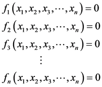
As it is well known from the basic principles of nonlinear algebra, a nonlinear system of n equations with n unknowns is defined as

(1)

or in vector form

(2)

where is the vector of the nonlinear functions each one of them being defined in the space of all real valued continuous functions and

(3)

is the vector of the system solutions (or roots). For the case of constant (namely non functional) coefficients, the above equations can also expressed as [6]

(4)

, where are the degrees of the above equations. It can be proven that this system has one non-vanishing solution (that is, at least one) if and only if the equation

(5)

holds, with the function to express the system resultant, a straightforward generalization of the determinant of a linear system. This function is a polynomial of the coefficients of A of degree

(6)

When all degrees coincide, that is, , the resultant is reduced to a simple polynomial of degree and it is described completely by the values of the parameters n and s. It can be proven that the coefficients of the matrix A, which is actually a tensor for n > 2, are not all independent to each other. More specifically, for the simple case, the matrix A is symmetric in the last s contra variant indices and it contains only independent coefficients, where

(7)

Even though the notion of the resultant has been defined for homogenous nonlinear equations, it can also describe non-homogenous algebraic equations as well. In the general case, the resultant satisfies the nonlinear Cramer rule

(8)

where is the component of the solution of the no homogenous system, and is the column of the coefficient matrix A.

The classical method for solving the nonlinear system defined above is the well known Newton’s method [7] that allows the approximation of the function by its first order Taylor expansion in the neighborhood of a point. This is an iterative method that uses as input an initial guess

(9)

and generates a vector sequence, with the vector associated with the iteration of the algorithm, to be estimated as

(10)

where is the Jacobian matrix of the function estimated at the vector x_k. Even though the method converges fast to the solution provided that the initial guess (namely the starting point x₀) is a good one, it is not considered as an efficient algorithm, since it requires in each step the evaluation (or approximation) of n² partial derivatives and the solution of an n × n linear system. A performance evaluation of the Newton’s method as well as other similar direct methods, shows that these methods are impractical for large scale problems, due to the large computational cost and memory requirements. In this work, besides the classical Newton’s method, the fixed Newton’s method was also used. As it is well known, the difference between these variations is the fact that in the fixed method the matrix of derivatives is not updated during iterations, and therefore the algorithm uses always the derivative matrix associated with the initial condition x₀.

An improvement to the classical Newton’s method can be found in the work of Broyden [8] (see also [9] as well as [10] for the description of the secant method, another well known method of solution), in which the computation at each step is reduced significantly, without a major decrease of the convergence speed; however, a good initial guess is still required. This prerequisite is not necessary in the well known steepest descent method, which unfortunately does not give a rapidly convergence sequence of vectors towards the system solution. The Broyden’s methods used in this work are the following:

・ Broyden method 1. This method allows the update of the Jacobian approximation B_i during the step i in a stable and efficient way and is related to the equation

(11)

where i and are the current and the previous steps of iterative algorithm, and furthermore we define, and.

・ Broyden method 2. This method allows the elimination of the requirement of a linear solver to compute the step direction and is related to the equation

(12)

with the parameters of this equation to be defined as previously.

3. Review of Previous Work

According to the literature [11] , the solution approaches for the nonlinear algebraic systems can be classified in two categories, namely the interval methods that are robust but too slow regarding their execution time, and the continuation methods that are suitable for problems where the total degree is not too high. The last years, a lot of different methods have been developed, in an attempt to overcome the limitations imposed by the classical algorithms and the related methods described above. An interesting and well known class of such methods, is the family of the ABS methods [12] that use a generalization of the projection matrices known as Abaffians ( [13] [14] , as well as [15] where the ABS methods are used in conjunction with the quasi-Newton method). There are also many other methods that are based on a lot of different approaches and tools, that among others include genetic algorithms [16] [17] , invasive weed optimization and stochastic techniques [18] [19] , fuzzy adaptive simulated annealing [20] , measure theory [21] , as well as neural networks [22] [23] and chaos optimization techniques [24] . The most important and recent of those methods are presented below.

Ren et al. [16] use a genetic algorithm approach to solve nonlinear systems of equations, in which a population of candidate solutions (known as individuals or phenotypes) to an optimization problem is evolved towards better solutions. Each candidate solution is associated with a set of properties (known as chromosomes or genotypes) that can be mutated and altered. In applying this algorithm, a population of individuals is randomly selected and evolved in time forming generations, whereas a fitness value is estimated for each one of them. In the next step, the more fit individuals are selected via a stochastic process and their genomes are modified to form a new population that is used in the next generation of the algorithm. The procedure is terminated when either a maximum number of generations has been produced, or a satisfactory fitness level has been reached.

In the work of Ren et al., the objective function to be minimized is the average of the absolute values of the functions , while the fitness function is defined as and in such a way, that the fitness value to be bigger if the point is closer to the solution of the problem. To improve the efficiency of this algorithm, it is mixed with the Newton’s method. On the other hand, El-Emary & El-Kareen [17] use a similar approach but their objective function is the maximum absolute value of the functions . For other approaches of solving nonlinear systems using genetic algorithms (see [25] and [26] ).

Pourjafari & Mojallali [18] attempt to solve a nonlinear system of equations via invasive weed optimization, a method that allows the identification of all real and complex roots as well as the detection of multiplicity. This optimization comprise four stages, namely 1) an initialization stage where a finite number of seeds are being dispread randomly on the n-dimensional search area as the initial solutions, 2) a reproduction stage where each plant is allowed to reproduce seeds based on its fitness with the number of seeds to increase linearly from the minimum possible seed production for the worst fitness, to the maximum number of seeds corresponding to the maximum fitness in the colony, 3) a spatial dispersal stage where the produced seeds are randomly distributed in the search space, such that they abide near to the parent plant by normal distribution with zero mean and varying variance and 4) a competitive exclusion, where undesirable plants with poor fitness are eliminated, whereas fitter plants are allowed to reproduce more seeds. This method is applied to the global optimization problem

(13)

with the root finding process to be composed of two phases, namely a global search where plants abandon non- minimum points vacant and settle down around minima, and an exact search where the exact locations of roots are determined via a clustering procedure that cluster plants around each root; in this way, the search is restricted only to that clusters.

Oliveira and Petraglia [20] attempt to solve nonlinear algebraic systems of equations via stochastic global optimization. The original problem is transformed into a global optimization one, by synthesizing objective functions whose global minima (if they exist) are also solutions to the original system. The global minimization is performed via the application of a fuzzy adaptive simulated annealing stochastic process, triggered from different starting points in order to find as many solutions as possible. In the method of Oliveira and Petraglia, the objective function is defined as the sum of the absolute values of the component functions and then it is submitted to the fuzzy adapted simulated annealing algorithm in an attempt to identify solutions for the above optimization problem. The algorithm is an iterative one and stops when an appropriately defined global error falls under a predefined tolerance value.

Effati and Nazemi [21] solved nonlinear algebraic systems of equations using the so-called measure theory, a tool capable of dealing with optimal control problems. In applying this theory, an error function is defined, the problem under consideration is transformed to an optimal control problem associated with the minimization of a linear functional over a set of Radon measures. In the next step, the optimal measure is approximated by a finite combination of atomic measures, the problem is converted approximately to a finite dimensional nonlinear programming and finally an approximated solution of the original problem is reached, together with a path leading from the initial problem to the approximate solution. On the other hand, Grosan and Abraham [27] deal the system of nonlinear equations as a multi-objective optimization problem. This problem tries to optimize the function subjected to a restriction in the form where is the solution search space. The algorithm proposed by Grosan and Abraham is an evolutionary computational technique consisting of an initialization and an optimization phase, with each one of the system equations to represent an objective function whose goal is to minimize the difference between the right and the left terms of the corresponding equation.

Liu et al. [28] used for solving nonlinear algebraic systems a variant of the population migration algorithm [29] that uses the well-known quasi-Newton method [9] . In applying the PAM algorithm to this problem, the

optimization vector x corresponds to the population habitual residence, the objective function

corresponds to the attractive place of residuals, whereas the global (local) optimal solution of the problems, corresponds to the most attractive (the beneficial) areas. Furthermore, the population flow corresponds to the local random search of the algorithm, while the population migration corresponds to the way of choosing solutions. The quasi-Newton variation of this approach, starts with a set of N uniformly and randomly generated points, and through an iterative procedure moves the most attract point to the center of the search region and shrinks that region until a criterion has been satisfied. At this point, the solution has been found.

The last family of methods used for the identification of nonlinear algebraic system roots is based to the use of neural network techniques. Typical examples of these methods include the use of recurrent neural networks [22] for the neural based implementation of the Newton’s method with the estimation of the Jacobian system matrix to be based on the properties of the sigmoidal activation functions of the output neurons, the use of the back propagation neural networks [30] for the approximation of the inverse function, as well as the neural computation method of Meng and Zeng [23] that uses an iterative algorithm and tries to minimize the objective function

(14)

where is an error function associated with the iteration of the algorithm, defined by the equation. Interesting methods for solving nonlinear algebraic systems using Hopfield neural networks and related structures can also be found in [31] and [32] .

Margaris, Goulianas and Adamopoulos [33] constructed four-layered feed forward neural nonlinear system solvers trained by the back propagation algorithm that uses fixed learning rate. The networks have been designed in such a way that the total input to a summation unit of the output layer to be equal to the left-hand side of the corresponding equation of the nonlinear system. In this way, the network is trained to generate the roots of the system, one root per training, with the components of the estimated root to be the variable weights of the synapses joining the unique input of the network with the n neurons of the first hidden layer, where n is the dimension of the non linear system. This network has been tested successfully in solving 2 × 2 [34] as well as 3 × 3 nonlinear systems [35] . Continuing this line of research, this paper generalizes earlier solvers for the general case of n × n nonlinear systems. This generalization is not restricted only to the dimension of the neural solver but it is extended to the form of the system (since it is capable of solving nonlinear systems of arbitrary equations and not only polynomial equations as its predecessors) whereas also supports the feature of an adaptive learning rate for the network neurons. The analytic description, simulation and performance evaluation of this neural architecture, is presented in the subsequent sections.

4. A Generalized Neural Nonlinear System Solver

In order to understand the logic behind the proposed method let us consider the complete 2 × 2 nonlinear algebraic system of equations

and the neural network of Figure 1. It is not difficult to note, that the outputs of the two output layer neurons are the functions and. These outputs are equal to zero if the values of the synaptic weights x and y are the roots of the nonlinear algebraic system, otherwise they are associated with a non zero value. Therefore, to estimate the system roots the two constant terms and are attached to the output neurons in the form of bias units and the hyperbolic tangent function is selected as their output function. Keeping in mind that the hyperbolic tangent of a zero value is the zero value, it is obvious that if we train the network using the vector as the desired output vector and the vector as the real output vector associated with each training cycle, then, after successful training, the variable synaptic weights x and y will contain by construction the components of one of the system roots. The same idea is used for the solution of the complete 3 × 3 nonlinear algebraic system studied in [35] .

The neural solver for the complete n × n nonlinear algebraic system is based exactly on the same logic, but there are also some new features that are not used in [34] and [35] . The most important feature is that the activation functions of the third layer neurons can be any function (such as trigonometric or exponential function) and not just a polynomial one, as in [34] and [35] , a feature that adds another degree of nonlinearity and allows the network to work correctly and with success, even though the activation function of the output neurons is a simple linear function. In this work, for the sake of simplicity this function is the identity function, while the case of the hyperbolic tangent function is a subject of future research. To allow a better formulation of the problem, the nonlinear function associated with the equation of the system is considered as a vector function in the form

(15)

where is the number of the function components associated with the vector function . Using this formalism the complete nonlinear algebraic system of n equations with n unknowns is defined as

Figure 1. The structure of neural network that solves the complete nonlinear algebraic system of two equations with two unknowns.

and its solution is the vector. Even though in this case the problem is defined in the field R of real numbers, its generalization in the field C of complex numbers is straightforward.

The neural network architecture that is capable of solving the general case of a n × n nonlinear system of algebraic equations, is shown in Figure 2 and is characterized by four layers with the following structure:

・ Layer 1 is the single input layer.

・ Layer 2 contains n neurons each one of them is connected to the input of the first layer. The weights of the n synapses defined in this way, are the only variable weights of the network. During network training their values are updated according to the equations of the back propagation and after a successful training these weights contain the n components of a system root

・ Layer 3 is composed of n blocks of neurons with the block containing neurons, namely, one neuron for each one of the functions associated with the equation of the nonlinear system. The neurons of this layer, as well as the activation functions associated with them, are therefore described using the double index notation for values and. This is a convenient way of description since a single numbering of all neurons requires the use of the MOD operator and adds further and unnecessary complexity to the mathematical description of the problem.

・ Layer 4 contains an output neuron for each equation, namely, a total number of n neurons that use the identity function as the activation function.

Figure 2. The proposed neural network architecture.

One the other hand, the matrices of the synaptic weights follow the logic used in [34] and [35] and they are defined as follows: The matrix

is the only variable weight matrix, whose elements (after the successful training of the network) are the components of one of the system roots, or in a mathematical notation .

The matrix W₂₃ is composed of n rows with the i_th row to be associated with the variable . The values of this row are the weights of the synapses joining the i_th neuron of the second layer with the complete set of neurons of the third layer. There is a total number of

neurons in this layer and therefore the dimensions of the matrix W₂₃ are. Regarding the values of these weights they have a value of unity if the function is a function of x_i, otherwise they have a zero value. Therefore, we have

(16)

Finally, the matrix W₃₄ has dimensions

with elements

(17)

The figure shows only the synapses with a nonzero weight value.

Since the unique neuron of the first layer does not participate in the calculations, it is not included in the index notation and therefore if we use the symbol u to describe the neuron input and the symbol v to describe the neuron output, the symbols u₁ and v₁ are associated with the n neurons of the second layer, the symbols u₂ and v₂ are associated with the k neurons of the third layer and the symbols u₃ and v₃ are associated with the n neurons of the third (output) layer. These symbols are accompanied by additional indices that identify a specific neuron inside a layer and this notation is used throughout the remaining part of the paper.

4.1. Building the Back Propagation Equations

In this section we build the equations of the back propagation algorithm. As it is well known form the literature, this algorithm is composed of three stages, namely a forward pass, a backward pass associated with the estimation of the delta parameter, and a second forward pass related to the weight adaptation process. In a more detailed description, these stages regarding the problem under consideration are performed as follows:

4.1.1. Forward Pass

The inputs and the outputs of the network neurons during the forward pass stage, are computed as follows:

LAYER 2 and .

LAYER 3 As it has been mentioned in the description of the neural system, since the neurons in the third layer are organized in n groups with the group to contain neurons, a double index notation is used with the index to identify the neuron group and the j index to identify a neuron inside the group. Using this convention and keeping in mind that when some variable appears in the defining equation of the associated activation function the corresponding input synaptic weight is equal to unity, the output of the neuron is simply equal to

(18)

LAYER 4 The input and the output of the fourth layer neurons are

(19)

and , where the activation function of the output neurons is the identity function.

4.1.2. Backward Pass―Estimation of d Parameters

In this backward phase of the back propagation algorithm the values of the δ parameters are estimated. The delta parameter of the neurons associated with the second, the third and the fourth layer is denoted as δ₁, δ₂ and δ₃, with additional indices to identify the position of the neuron inside the layer. Starting from the output layer and using the well known back propagation equations we have

(20)

On the other hand, the delta parameter of the third layer neurons are

Note that, in this case, for each third layer neuron and for each one of the x_k parameters (where), the values of n derivatives are estimated.

Finally, the δ parameter of the second layer neurons have the form

where we use the notation

(21)

In the last two equations the j variable gets the values.

5. Convergence Analysis and Update of the Synaptic Weights

By the mean square error defining equation

where is the desired output of the neuron of the output layer and is the corresponding real output, we have

(22)

. By applying the update weight equation of the back propagation, we get

(23)

where is the learning rate of the back propagation algorithm and and are the values of the synaptic weight during the and iteration.

The Case of Adaptive Learning Rate

The adaptive learning rate is a novel feature of the proposed simulator that allows each neuron of the second layer to have its own learning rate. However, these learning rate values must ensure the convergence of the algorithm, and the allowed range for those values has to be identified. This task can be performed based on energy considerations.

The energy function associated with the iteration is defined as

If the energy function for the iteration is denoted as, the energy difference is

From the weight update equation of the back propagation algorithm we have

(24)

and therefore,

. Using this expression in the equation of, it gets the form

The convergence condition of the back propagation algorithm is expressed as. Since we have (the learning value is obviously a positive number) and of course it holds that

(25)

it has to be

(26)

or equivalently

(27)

Defining the adaptive learning rate parameter (ALRP) μ, the above equation can be expressed as

(28)

where is the k_th column of the Jacobian matrix

(29)

for the m_th iteration. Using this notation, the back propagation algorithm converges for adaptive learning rate parameter (LALR) values μ < 2.

6. Experimental Results

To examine and test the validity and the accuracy of the proposed method, sample nonlinear algebraic systems were selected and solved using the neural network approach and the results were compared against those obtained from other methods. More specifically, the network solved five nonlinear example systems of n equations with n unknowns, three systems for n = 2, one system for n = 3 and one system for n = 6. In these simulations, the adaptive learning rate approach (ALR) is considered as the primary algorithm, but the network is also tested with a fixed learning rate (FLR) value. Even though in the theoretical analysis and the construction of the associated equations the classical back propagation algorithm was used, the simulations showed that the execution time can be further decreased (leading to the speedup of the simulation process) if in each cycle the synaptic weights were updated one after the other and the new output values were used as input parameters in the corrections associated with the next weight adaptation, an approach that is also used by Meng & Zeng [23] . The results of the simulation for the ALR approach are presented using graphs and tables, while the results for the FLR case are presented in a descriptive way. Since the accuracy of the results found in the literature varies significantly, and since the comparison of the root values requires the same number of decimal digits, different tolerance values in the form 10^−tol were used, with a value of tol = 12 to give an accuracy of 6 decimal digits (as in the work of Effati & Nazemi [21] and Grosan & Abraham [27] ), a value of tol = 31 to give an accuracy of 15 decimal digits (as in the work of Oliveira & Petraglia [20] ) and a value of tol = 20 to give an accuracy of 10 decimal digits (as in the work of Meng & Zeng [23] and Liu et al. [28] ).

According to the proposed method, the condition that ensures the convergence of the back propagation algorithm is given by the inequality μ < 2, where μ is the adaptive learning rate parameter (ALRP). Therefore, to test the validity of this statement, a lot of simulations were performed, with the value of ALRP varying between μ = 0.1 and μ = 1.9 with a variation step equal to 0.1 (note, however, that the value μ = 1.95 was also used). The maximum allowed number of iterations was set to N = 10000 and a training procedure that reaches this limit is considered to be unsuccessful. In all cases, the initial conditions is a set in the form and the search region is an n-dimensional region defined as

In almost all cases, the variation step of the system variables is equal to 0.1 or 0.2 even though the values of 0.5 and 1.0 were also used for large values to reduce the simulation time. The graphical representation of the results shows the variation of the minimum iteration number with respect to the value of the adaptive learning rate parameter μ; an exception to this rule is the last system, where the variable plotted against the μ parameter is the value of the algorithm success rate.

After the description of the experimental conditions let us now present the five example systems as well as the experimental results emerged for each one of them. In the following presentation the roots of the example systems are identified and compared with the roots estimated by the other methods.

Example 1: Consider the following nonlinear algebraic system of two equations with two unknowns:

This system has a unique root with a value of

Note, that this example can also be found in the papers of Effati & Nazemi [21] , Grosan & Abraham [27] and Oliveira & Petraglia [20] .

The experimental results for this system and for are presented in Table 1 and Table 2. The results in Table 1 have been computed with a tolerance value tol = 12, while the results in Table 2 are associated with a tolerance value tol = 31. In the first case, the best result is associated with the ALRP value μ = 1.1, initial conditions and it was reached after N = 7 iterations of the back propagation algorithm. In the second case the best result is associated again with the ALRP value μ = 1.1 and initial conditions, but it was reached after N = 32 iterations.

Example 2: This system includes also two equations with two unknowns and it is defined as

and it has infinite roots. Therefore, in this case the neural solver tries to identify those roots that belong to the search interval used in any case. This system is also examined in the papers of Effati & Nazemi [21] , Grosan & Abraham [27] and Oliveira & Petraglia [20] .

The experimental results in this case are the identified roots in the intervals for values α = 2, 10, 100, 1000. The system solving procedure found a lot of roots, and this is an advantage over the other methods, since they found only one root (note, that this is not the case with the system of the Example 1, since by construction, it has a unique root). More specifically, the system has 1 root in the interval [−2, +2], 13 roots in the interval [−10, +10], 127 roots in the interval [−100, +100] (these numbers of roots are also reported by Tsoulos & Stavrakoudis [36] , who also examined the same example system without reporting their identified root values to make a comparison) and 1273 roots in the interval [−1000, 1000]. It is interesting to note that, besides these roots, the neural network was able to identify additional roots, located outside the search interval used in any

Table 1. The experimental results for the first example system (ALR, Effati & Nazemi and Grosan & Abraham methods).

Table 2. The experimental results for the first example system (ALR and Oliveira & Petraglia methods).

case; these roots are not reported in the results, since they are identified again in the next simulation, where the value of the α parameter increases. For example, for μ = 0.5 and α = 2, the network found 23 roots but we keep only the root, since only this root belongs to the search region −2 ≤ x₁, x₂ ≤ 2. In the same way, for α = 10 and for the same μ value, the network found 149 roots, but only 13 of them belong to the search interval −10 ≤ x₁, x₂ ≤ 10. It is not difficult to guess, that the 23 roots found for α = 2 is a subset of the 149 roots found for α = 10, and so on. The simulation results for α = 2 associated with a tolerance value of tol = 12 and tol = 31 are shown in Table 3 and Table 4, and the associated plot is shown in Figure 3. The number of identified roots that belong to the search region for α = 2, 10, 100 as well as the percentage of those roots with respect to the total number of identified roots for that region, are shown in Table 5. The values of the 13 identified roots that belong to the search region −10 ≤ x₁, x₂ ≤ 10 with 15 digits accuracy, namely for a tolerance of tol = 31, are shown in Table 6. The variation of the minimum iteration number with the parameter μ for each one of the 13 identified roots for the case α = 10 is shown in Figure 4, while Figure 5 shows the percentage of initial condition combinations associated with identified roots that belong to the search region for the parameter values α = 2, 10, 100. The total number of the examined systems was 441 for α = 2 (namely −2 ≤ x₁, x₂ ≤ 2 with variation step Δx₁ = Δx₂ = 0.2), 10,201 for α = 10 (namely −10 ≤ x₁, x₂ ≤ 10 with variation step Δx₁ = Δx₂ = 0.2) and 10,201 for α = 100 (namely −100 ≤ x₁, x₂ ≤ 100 with variation step Δx₁ = Δx₂ = 0.2).

The results for α = 1000 are too lengthy to be presented here and, due to the enormous computation time, it was not possible to perform the exhaustive search as with the previous cases. Therefore, the algorithm run with variation steps of Δx₁ = Δx₂ = 0.2, 0.5 and 1.0, and only for the ALRP value μ = 1.5. The number of identified roots in each case varies according to the variation step, but in all cases the network identified a number of 1273 roots in the interval [−1000, +1000]. This is a new result that does not appear in the other works used for comparison.

Before proceeding to the next example system, let us present some results regarding the FLR (fixed learning rate) method, in which all the neurons share the same learning rate value. In this experiment the learning rate

Figure 3. Simulation results for the example 2 for tolerance tol = 12 and tol = 31.

Table 3. The experimental results for the second example system and for α = 2 (ALR, Effati & Nazemi and Grosan & Abraham methods).

Table 4. The experimental results for the second example system and for α = 2 (ALR and Oliveira & Petraglia methods).

Table 5. The number of the identified roots and the associated percentage of roots that belong to the search region for the values α = 2, 10, 100 and for a tolerance value of 10⁻¹².

Table 6. The values of the 13 roots found in the search region −10 ≤ x₁ ≤ 10 and −10 ≤ x₂ ≤ 10 with an accuracy of 15 decimal digits, namely for a tolerance value of 10⁻³¹.

Figure 4. Variation of the minimum iteration number with respect to the value of the parameter for each one of the 13 roots found in the interval [−10, +10] for the second example system. Due to the large variation of the minimum iteration number, the vertical axis follows the logarithmic scale. The numbering of roots is the same as in Table 6.

Figure 5. Variation of the percentage of initial conditions leading to system roots that belong to the search region with respect to the value of the ALRP parameter for α = 2, 10, 100.

was much smaller than ALR, with the μ parameter to get the values from μ = 0.01 to μ = 0.2, with a variation step of Δμ = 0.1. The tolerance value was equal to tol = 12 and the systems studied for the parameters α = 2, 10, 100. As a typical example, let us present the results associated with the value μ = 0.11. In this case, the network identified the unique root for α = 2 (as well as 4 additional roots outside the search region) after 17 iterations and 127 roots for α = 100 (as well as 24 additional roots outside the search interval), and for the same iteration number. The simulation showed that the performance of the network decreases as the FLR value varies from 0.15 to 0.2 (with a variation step of 0.01). More specifically, in this case, the neural network is not able to identify the unique root in the interval [−2, 2] and, furthermore, it finds only the half of the roots found previously (namely, 6 of 13 roots in the interval [−10, 10] and 64 of 127 roots in the interval [−100, 100]). A construction of a diagram similar to the one shown in Figure 3 and Figure 4, would reveal that for the second example system the best FLR value is the value μ = 0.14, associated with 31 iterations. The basin of attraction for the 13 identified roots associated with the value α = 10 and for a fixed learning rate with a value of FLR = 0.02 is shown in Figure 6.

Example 3: This nonlinear algebraic system can be found in [23] and is composed again of two equations with two unknowns. More specifically, the system is defined as

and it has a unique root with a value of

It is interesting to note that the solution method proposed for this system in the literature, is also a neural based approach and, therefore, it is more suitable for comparison with the proposed method. The simulation results emerged from the proposed neural method, as well as from the method of Meng & Zeng are shown in Table 7. In this table the results are associated with four distinct sets of initial conditions, namely . In order to estimate the roots with an accuracy of 9 digits, a tolerance value of tol = 20 was used. The table also includes the values of the vector norm. The variation of the minimum iteration number for the example system 3 with the ALRP parameter is shown in Figure 7 and, as it can be easily verified, the ALRP value that gives the best results is μ = 1.1 (the same value is also reported in [23] ). Regarding the ALRP value of 1.1 that gave the best results, the minimum, the maximum and the average iteration numbers are equal to 9, 13 and 11.675 iterations respectively.

Example 4: Consider the system of three equations with three unknowns defined as

This system has only one root. The solution of this system using the Population Migration Algorithm (PAM) [29] as well as its variant known as Quasi-Newton PAM (QPAM) is given by Liu et al. [28] . To test this result and

Figure 6. Basin of attraction for the 13 identified roots for the system of the Example 2, for α = 10 and for a fixed learning rate with value FLR = 0.02.

Table 7. Simulation results for the example system 3.

Figure 7. Variation of the minimum iteration number with respect to the value of the parameter for the example system 3 in the interval [−2, +2].

evaluate the performance of the proposed neural solver, the system is solved for the search region −2 ≤ x₁, x₂, x₃ ≤ 2 with a variation step of Δx₁ = Δx₂ = Δx₃ = 0.2, leading thus to the examination of 9261 initial condition combinations. For each one of those combinations the root identification was performed using the same ALRP values (namely from μ = 0.1 to μ = 1.95). The results for the best simulation runs can be found in Table 8, together with the results of Liu et al. for comparison purposes. From this table it is clear that the best result with respect to the success rate is associated with the value μ = 0.7, while the best value with respect to the minimum iteration number is associated with the value μ = 1.1.

A typical graph that shows the variation of the average iteration number with respect the value of the ALRP parameter is shown in Figure 8. Similar graphs can be constructed for each example presented in this section and the above mentioned variation in all cases follows a similar pattern.

Example 5: The last example is associated with a large enough nonlinear algebraic system of six equations with six unknowns defined as

Table 8. Simulation results for the example system 4 (Example 8 of Liu et al.).

Figure 8. Variation of the average iteration number with respect to the value of the parameter for the example system 4 in the interval [−2, +2].

This system also appears in the work of Liu et al. [28] and it has an optimum solution with a value of x₁ = x₃ = x₅ = −1 and x₂ = x₄ = x₆ = 1. The experimental results for this system are given in Table 9, together with the results of the algorithms PMA and QPMA. From this table it is clear that the best result with respect to the iteration number is associated with the ALRP value μ = 1.5 (63 iterations with a success rate of 71%). Note, that it is possible to improve significantly the success rate using a smaller ALRP value, but with a significant increase of the computational cost (for example the value μ = 0.1 gives a success rate of 92% but after 6037 iterations). The corresponding results for fixed learning rate are (μ = 1.0, 81 iterations with 6% success rate) and (μ = 0.005, 7468 iterations with 78% success rate). Note that for all values of the adaptive learning rate and a fixed learning rate value less than 0.5 the network identifies and a second solution that does not belong to the search interval with a value of

Table 9.Simulation results for the example system 4 (Example 9 of Liu et al.).

The variation of the success rate with respect to the ALRP parameter μ for the last two example systems is plotted in Figure 9.

Figure 9. The variation of the success rate with the value of parameter for the Example Systems 4 and 5.

Test Results with Iteration Number and Execution CPU Time for Large Sparse Nonlinear Systems of Equations

A very crucial task in evaluating this type of arithmetic methods is to examine their scaling capabilities and more specifically to measure the iteration number and the execution time as the dimension of the system increases. In order to compare the results of the proposed method with the ones emerged by other well known methods, the following example systems were implemented and solved using the proposed algorithm:

・ Example 6: This system is Problem 1 in [37] and it is defined as

with initial conditions.

・ Example 7: This system is Problem 3 in [37] and it is defined as

with initial conditions

・ Example 8: This system is Problem 4 in [37] and it is defined as

with initial conditions

・ Example 9: This system is Problem 2 in [38] and it is defined as

with initial conditions and parameter value h = 2.

・ Example 10: This system is Problem 1 in [38] and it is defined as

with initial conditions.

・ Example 11: This system is Problem 2 in [39] and it is defined as

with initial conditions.

・ Example 12: This system is Problem 3 in [40] and it is defined as

with initial conditions.

・ Example 13: This system is Problem 5 in [40] and it is defined as

with initial conditions.

The stopping criterion in these simulations is defined as

(30)

where tol is the tolerance value. To achieve the best results and an accuracy of 6 decimal points in the final solution, different values for tol and ALRP were used in each example, and more specifically,

・ the values tol = 12 and ALRP = 19 for Example 6

・ the values tol = 12 and ALRP = 0.8 for Example 7

・ the values tol = 12 and ALRP = 1.0 for Example 8

・ the values tol = 12 and ALRP = 0.6 for Example 9

・ the values tol = 18 and ALRP = 1.1 for Example 10

・ the values tol = 36 and ALRP = 1.9 for Example 11

・ the values tol = 10 and ALRP = 0.8 for Example 12

・ the values tol = 12 and ALRP = 1.0 for Example 13

The simulation results for the above examples are summarized in Table 10. For each example the system dimension n was set to the values 5, 10, 20, 50, 100, 200, 500 and 1000. In this table, a cell with the “-” symbol means that either the algorithm could not lead to a result (i.e. it was divergent), or the maximum number of iterations (with a value equal to 500) was reached. This is especially true for the Examples 9 and 10, where the only method capable of reaching a result, was the proposed method (GBARL i.e. Generalized Back-propagation with Adaptive Learning Rate). It also has to be mentioned that the Examples 8 are 13 were run twice. In Example 8, the first run (Example 8a) was based on the initial condition , while the second run (Example 8b) used the initial condition vector (see [41] ) with parameter values ALR = 1.0 and tol = 10. In the same way, in Example 13 the two runs are based on the initial condition vectors (Example 13a with ALR = 1.0 and tol = 12) and (Example 13b with ALR = 0.8 and tol = 12).

The simulation runs were implemented on an Intel Core i5 cpu machine with 2.66Ghz and 4GB Memory, the applications were written in Matlab and the main conclusions drawn from them are the following:

・ In most of the examples (except examples 8a and 9), the iteration number is almost the same, no matter the dimension of the systems used.

・ In most of the examples, the proposed method needs less iterations than Newton and Broyden methods even for the large systems, and is better in CPU time for the convergence to a good solution with 6 decimal points accuracy, except the case of n ≥ 200, where Broyden-2 method has better CPU time.

・ In Example 8a the Newton method converges only for small dimensions, and for values n ≥ 5 the only method that converges is the proposed one.

Table 10. Tables for Examples 6-13 with Iteration number and CPU time (in seconds) for systems with n = 50,10, 20, 50, 100, 200, 500, 1000, using Newton, Fixed Newton, Broyden-1, Broyden-2 and GBALR methods.

・ In Examples 7, 9 and 10 the proposed method (GBARL) is the only that converges.

・ The fixed Newton method converges only in Examples 8b, 12 and 13b.

・ In Example 12 the proposed method needs only one iteration to converge.

・ Even though the Broyden-2 method leads generally to better CPU times for large system dimensions (e.g. n = 200), in a lot of cases it is unable to converge (e.g. in Examples 7, 8, 9, 10).

・ In Example 8a the proposed method exhibits an irregular behavior regarding the variation of the iteration number, while in Example 9 this variation is more regular. In all the other cases, the number of iterations is almost constant with a very small variations.

・ Besides the Examples 8b and 13, the required number of iterations for convergence is smaller than the one associated with the other methods.

7. Conclusion

The objective of this research was the design and performance evaluation of a neural network architecture, capable of solving a complete nonlinear algebraic system of n equations with n unknowns. The developed theory shows that the network must be used with an adaptive learning rate parameter μ < 2. According to the experiments, for small values of the system dimension n, good values of μ can be found in the region [0.7, 1.7] with a best value at μ < 1.1, whereas for large n, good values of μ can be found in the region [1.0, 1.9], with a best value at μ < 1.5. The network was able to identify all the available roots in the search region with an exceptional accuracy. The proposed method was tested with large sparse systems with dimension from n = 5 to n = 1000 and in the most cases the number of iterations did not depend on the system dimension. The results showed that the GBARL method was better than the classical methods with respect to the iteration number required for convergence to a solution, as well as the CPU execution time, for system dimensions n ≤ 100. Regarding larger system dimensions, the GBARL method is better than the Broyden-2 method with respect to the number of iterations but requires more CPU execution time. However the Broyden-2 could not able to converge for a lot of examples and for the initial conditions found in the literature. Challenges for future research include the use of the network with other activation functions in the output layer, such as the hyperbolic tangent function, as well as the ability of the network to handle situations such that the case of multiple roots (real and complex) for the case of overdetermined and underdetermined systems.

Acknowledgements

The research of K. Goulianas, A. Margaris, I. Refanidis, K. Diamantaras and T. Papadimitriou, has been co-financed by the European Union (European Social Fund-ESF) and Greek national funds through the Operational Program “Education and Lifelong Learning” of the National Strategic Reference Framework (NSRF)― Research Funding Program: THALES, Investing in knowledge society through the European Social Fund.

Conflicts of Interest

The authors declare no conflicts of interest.

References

[1]	Zhang, G. and Bai, L. (2009) Existence of Solutions for a Nonlinear Algebraic System. Discrete Dynamics in Nature and Society, 2009, Article ID: 785068.
[2]	Kowalski, K. and Tankowski, K. (1998) Towards Complete Solutions to Systems of Nonlinear Equations of Many-Electron Theories. Physical Review Letters, 81, 1195-1998. http://dx.doi.org/10.1103/PhysRevLett.81.1195
[3]	Holstad, A. (1999) Numerical Solution of Nonlinear Equations in Chemical Speciation Calculations. Computational Geosciences, 3, 229-257. http://dx.doi.org/10.1023/A:1011595429513
[4]	Argyros, K. (1993) On the Solution of Underdetermined Systems of Nonlinear Equations in Euclidean Spaces. Pure Mathematics and Applications, 4, 199-209.
[5]	Morgan, A.P. (1987) Solving Polynomial Systems Using Continuation for Scientific and Engineering Problems. Prentice-Hall, Eaglewood Cliffs.
[6]	Dolotin, V. and Morozov, A. (2007) Introduction to Non-Linear Algebra. World Scientific Publishing Company, Singapore. http://dx.doi.org/10.1142/6508
[7]	Burden, R.L. and Faires, J.D. (2010) Numerical Analysis. Brooks Cole, Pacific Grove.
[8]	Broyden, C.G. (1965) A Class of Methods for Solving Nonlinear Simultaneous Equations. Mathematical Computations, 19, 577-593. http://dx.doi.org/10.1090/S0025-5718-1965-0198670-6
[9]	Broyden, C.G., Dennis, J.E. and More, J.J. (1973) On the Local and Superlinear Convergence of Quasi-Newton Methods. IMA Journal of Applied Mathematics, 12, 223-245. http://dx.doi.org/10.1093/imamat/12.3.223
[10]	Dennis, J.E. and Wolkowicz, H. (1993) Least Change Secant Methods, Sizing, and Shifting. SIAM Journal on Numerical Analysis, 30, 1291-1314.
[11]	Hentenryck, P., McAllester, D. and Kapur, D. (1997) Solving Polynomial Systems Using a Branch and Prune Approach. SIAM Journal on Numerical Analysis, 34, 797-827. http://dx.doi.org/10.1137/S0036142995281504
[12]	Abaffy, J. and Spedicato, E. (1989) ABS Projection Algorithms: Mathematical Techniques for Linear and Nonlinear Equations. Ellis Horwood, Hemel Hemstead.
[13]	Abaffy, J. and Galantai, A. (1987) Conjugate Direction Methods for Linear and Nonlinear Systems of Algebraic Equations. Numerical Methods, 50, 481-502.
[14]	Abaffy, J., Galantai, A. and Spedicato, E. (1987) The Local Convergence of ABS Methods for Nonlinear Algebraic Equations. Numerische Mathematik, 51, 429-439. http://dx.doi.org/10.1007/BF01397545
[15]	Galantai, A. and Jeney, A. (1996) Quasi-Newton ABS Methods for Solving Nonlinear Algebraic Systems of Equations. Journal of Optimization Theory and Applications, 89, 561-573. http://dx.doi.org/10.1007/BF02275349
[16]	Ren, H., Wu, L., Bi, W.H. and Argyros, I.K. (2013) Solving Nonlinear Equations System via an Efficient Genetic Algorithm, with Symmetric and Harmonious Individuals. Applied Mathematics and Computation, 219, 10967-10973.
[17]	El-Emary, I.M.M. and El-Kareem, M.M.A. (2008) Towards Using Genetic Algorithms for Solving Nonlinear Equation Systems. World Applied Sciences Journal, 5, 282-289.
[18]	Pourjafari, E. and Mojallali, H. (2012) Solving Nonlinear Equation Systems with a New Approach Based on Invasive Weed Optimization Algorithm and Clustering. Swarm and Evolutionary Computation, 4, 33-43. http://dx.doi.org/10.1016/j.swevo.2011.12.001
[19]	Mehrabian, A.R. and Lucas, C. (2006) A Novel Numerical Optimization Algorithm Inspired from Weed Colonization. Ecological Informatics, 1, 355-366. http://dx.doi.org/10.1016/j.ecoinf.2006.07.003
[20]	Oliveira, H.A. and Petraglia, A. (2013) Solving Nonlinear Systems of Functional Equations with Fuzzy Adaptive Simulated Annealing. Applied Soft Computing, 13, 4349-4357. http://dx.doi.org/10.1016/j.asoc.2013.06.018
[21]	Effati, S. and Nazemi, A.R. (2005) A New Method for Solving a System of the Nonlinear Equations. Applied Mathematics and Computations, 168, 877-894. http://dx.doi.org/10.1016/j.amc.2004.09.029
[22]	Mathia, K. and Saeks, R. (1995) Solving Nonlinear Equations Using Recurrent Neural Networks. Proceedings of World Congress on Neural Networks (WCNN’95), Washington DC, 17-21 July 1995, 76-80.
[23]	Meng, A. and Zeng, Z. (2011) A Neural Computational Method to Solve Nonlinear Equation Systems. Journal of Computational Information Systems, 7, 3462-3469.
[24]	Luo, Y.Z., Tang, G.T. and Zhou, L.N. (2008) Hybrid Approach for Solving Systems of Nonlinear Equations Using Chaos Optimization and Quasi-Newton Method. Applied Soft Computing, 8, 1068-1073. http://dx.doi.org/10.1016/j.asoc.2007.05.013
[25]	Kuri-Morales, A.F. (2003) Solution of Simultaneous Nonlinear Equations Using Genetic Algorithms. WSEAS Transactions on Systems, 2, 44-51.
[26]	Nasira, G.N. and Devi, D.S. (2012) Solving Nonlinear Equations through Jacobian Sparsity Patterns Using Genetic Algorithms. International Journal of Communications and Engineering, 5, 78-82.
[27]	Grosan, C. and Abraham, A. (2008) A New Approach for Solving Nonlinear Equation Systems. IEEE Transactions on Systems, Man, and Cybernetics, Part A: Systems and Humans, 38, 698-714. http://dx.doi.org/10.1109/TSMCA.2008.918599
[28]	Liu, H., Zhou, Y. and Li, Y. (2011) A Quasi-Newton Population Migration Algorithm for Solving Systems of Nonlinear Equations. Journal of Computers, 6, 36-42. http://dx.doi.org/10.4304/jcp.6.1.36-42
[29]	Zhou, Y.H. and Mao, Z.Y. (2003) A New Search Algorithm for Global Optimization—Population Migration Algorithm. Journal of South China University of Technology, 21, 1-5.
[30]	Zhao, Q. and Li, W. (2012) An Improved Iterative Algorithm of Neural Network for Nonlinear Equation Groups. Proceedings of IEEE 2nd International Conference on Business Computing and Global Informatization, Shanghai, 12-14 October 2012, 522-525. http://dx.doi.org/10.1109/bcgin.2012.142
[31]	Mishra, D. and Kalra, P.K. (2007) Modified Hopfield Neural Network Approach for Solving Nonlinear Algebraic Equations. Engineering Letters, 14, 135-142.
[32]	Li, G. and Zeng, Z. (2008) A Neural-Network Algorithm for Solving Nonlinear Equation Systems. 9th International Conference on Computational Intelligence and Security, 1, 20-23. http://dx.doi.org/10.1109/cis.2008.65
[33]	Margaris, A. and Adamopoulos, M. (2007) Solving Nonlinear Algebraic Systems Using Artificial Neural Networks. Proceedings of the 10th International Conference on Engineering Applications of Artificial Neural Networks, Thessaloniki, 29-31 August 2007, 107-120.
[34]	Margaris, A. and Goulianas, K. (2012) Finding All Roots of 2 × 2 Nonlinear Algebraic Systems Using Back-Propagation Neural Networks. Neural Computing and Applications, 21, 891-904. http://dx.doi.org/10.1007/s00521-010-0488-z
[35]	Goulianas, K., Margaris, A. and Adamopoulos, M. (2013) Finding All Real Roots of 3 × 3 Nonlinear Algebraic Systems Using Neural Networks. Applied Mathematics and Computation, 219, 4444-4464. http://dx.doi.org/10.1016/j.amc.2012.10.049
[36]	Tsoulos, I.G. and Stavrakoudis, A. (2010) On Locating All Roots of Systems of Nonlinear Equations inside Bounded Domain Using Global Optimization Methods. Nonlinear Analysis: Real World Applications, 11, 2465-2471. http://dx.doi.org/10.1016/j.nonrwa.2009.08.003
[37]	Waziri, M.Y., Leong, W.J. and Mamat, M. (2012) A Two-Step Matrix-Free Secant Method for Solving Large-Scale Systems of Nonlinear Equations. Journal of Applied Mathematics, 2012, Article ID: 348654.
[38]	Leong, W.J., Hassan, M.A. and Yusuf, M.W. (2011) A Matrix-Free Quasi-Newton Method for Solving Large-Scale Nonlinear Systems. Computers and Mathematics with Applications, 62, 2354-2363. http://dx.doi.org/10.1016/j.camwa.2011.07.023
[39]	Yu, G., Niu, S., Ma, J. and Song, Y. (2013) An Adaptive Prediction-Correction Method for Solving Large-Scale Nonlinear Systems of Monotone Equations with Applications. Abstract and Applied Analysis, 2013, Article ID: 619123.
[40]	Mamat, M., Muhammad, K. and Waziri, M.Y. (2014) Trapezoidal Broyden’s Method for Solving Systems of Nonlinear Equations. Applied Mathematical Sciences, 8, 251-260.
[41]	Sun, W. and Yuan, Y-X. (2006) Optimization Theory and Methods, Nonlinear Programming. Springer, New York.