Properties of Solutions of Kolmogorov-Fisher Type Biological Population Task with Variable Density ()
Received 5 April 2016; accepted 20 May 2016; published 23 May 2016

1. Introduction
Population models are studied for a long time. The first such work was done by Gause G.F. and Fisher R.D., and mathematical studies were performed by Kolmogorov, Petrovskii (KPP) and Piskunov (1937) in the famous paper [1] - [4] . They were interested in the behavior of the speed of the wave solutions and the resulting estimate of the speed of wave propagation.
Then there were other models of the population [5] - [8] . In recent years, intensive study of nonlinear models was based on diffusion and revealed new properties of finite speed of propagation of diffusion waves (see [3] and the literature given there). We have proposed a population model of two competing populations with non-linear double diffusion and variable density that are described by nonlinear system of competing individuals. We identify new properties, such as finite speed of propagaton, and localization of the outbreaks in a specific area. In particular, in the critical case, the rate type CPT generalizes their result.
Statement of the Task
In this paper, we investigate the properties of solutions of biological population task of Fisher-Kolmogorov type in the case of variable density. The main research method is a self-similar approach. Considering in the field , there is a parabolic system of two quasilinear equations of reaction-diffusion
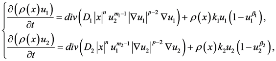 (1)
(1)
 ,
,  , (2)
, (2)
which describes the process of biological population of Kolmogorov-Fisher in a nonlinear two-component environment, and mutual diffusion coefficients which are respectively equal to ,
,  . Numeric parameters
 ,
,  ,
,  are positive real numbers, and
 ,
,  ,
,  ,
,
 ;
; ,
, ![]() is desired solutions.
is desired solutions.
We study properties of solutions to problem (1), (2) based on the self-similar analysis of solutions of a system of equations constructed by the method of nonlinear splitting and a reference equations and bringing the system (1) for radially symmetric mind. Note that replacing in (1)
![]() ,
, ![]()
leads to the form
![]() (3)
(3)
![]() ,
,![]() . (4)
. (4)
If![]() , choosing
, choosing
![]() ,
, ![]() ,
, ![]() ,
,
we get the following system of equations:
![]() (5)
(5)
where![]() ,
, ![]()
![]() ,
, ![]()
If![]() , and
, and![]() ,
, ![]() , system has the form:
, system has the form:
![]() (6)
(6)
A significant role in the study of the Cauchy problem and boundary problems for Equations (1) has self- similar solutions. Under self-similar solution we will understand as particular solutions of Equation (1), depending on the combination of t and x. Knowledge of them plays a sometimes crucial role in the study of various properties of solutions of the original equations.
Below we describe one way of obtaining self-similar system for the system of Equations (5). It consists in the following. We find first the solution of a system of ordinary differential equations
![]()
in the form
![]() ,
, ![]() ,
,
for the case of![]() , and
, and![]() ,
,![]() . And in the case of
. And in the case of![]() , and
, and![]() ,
, ![]() we solve a system of ordinary differential equations
we solve a system of ordinary differential equations
![]()
in the form
![]() ,
, ![]() ,
,
then the solution of system (5) is sought in the form
![]() (7)
(7)
and ![]() is selected so
is selected so
![]()
if![]() .
.
Then for ![]() we get the system of equations:
we get the system of equations:
![]() (8)
(8)
where
![]() (9)
(9)
![]()
If![]() , self-similar solution of system (9) has the form
, self-similar solution of system (9) has the form
![]() , (10)
, (10)
Then substituting (10) into (8) with respect to ![]() gets a self-similar system of equations
gets a self-similar system of equations
![]() (11)
(11)
where ![]() и
и![]() .
.
System (11) has an approximate solution of the form
![]() ,
, ![]() ,
,
where А and В are constants and
![]() ,
,![]() .
.
In this paper, on the basis of the aforesaid methods, we studied qualitative properties of solutions of the system (1), solved the problem of choosing the initial approximation for iterative, leading to fast convergence to the solution of the Cauchy problem (1), (2), depending on the values of numerical parameters and initial data. For this purpose, as the initial approximation was used, we found the asymptotic representation of the solution. This has allowed to perform numerical experiments and visualization of the process described by system (1), depending on the values included in the system of numeric parameters.
2. Construction of Upper Solutions
Let us build an upper solution for system (11).
Note that the functions ![]() have properties
have properties
![]()
and
![]()
We choose A and B from the system of nonlinear algebraic equations
![]()
Then functions ![]() were the solution of the Zel’dovich-Kompanees for the system (1) and in the field
were the solution of the Zel’dovich-Kompanees for the system (1) and in the field ![]() they satisfy the system of equations
they satisfy the system of equations
![]()
in the classical sense.
Due to the fact that
![]()
function ![]() and the flows have the following smoothness properties
and the flows have the following smoothness properties
![]()
![]() .
.
We choose A and B such that the inequality of inequality
![]() (12)
(12)
Since then
![]()
It is due to the fact that
![]()
from (12) we have
![]()
Then in the field Q according to the comparison principle of solutions have
Theorem 1. Let ![]() Then for the solution of problem (1) Q is the evaluation
Then for the solution of problem (1) Q is the evaluation
![]()
![]()
where![]() ―above-defined functions.
―above-defined functions.
Note that the solution of system (1) when ![]() has the following representation at
has the following representation at
![]()
where B(a, b)-Euler Beta function.
It is proved that this view is the self-similar asymptotics of solutions of systems (1).
![]()
![]()
Here
![]()
3. Slow Diffusion
Case ![]() (slow diffusion). Applying the method of [1] to solve Equation (11) will receive the following features
(slow diffusion). Applying the method of [1] to solve Equation (11) will receive the following features
![]()
where![]() ,
, ![]() ,
,![]() . It is known [1] [2] that for the global existence of solutions of problem (1) function
. It is known [1] [2] that for the global existence of solutions of problem (1) function ![]() must satisfy the following inequality:
must satisfy the following inequality:
![]()
and
![]() .
.
Let’s take the function![]() , and show that they are asymptotic finite solutions of the system (11).
, and show that they are asymptotic finite solutions of the system (11).
Theorem 2. The finite solution of system (11) when ![]() has asymptotic
has asymptotic![]() .
.
Proof. We seek a solution of Equation (8) in the following form
![]() , (13)
, (13)
where![]() , and
, and ![]() at
at![]() , to explore the asymptotic stability of the solution of problem (11) when
, to explore the asymptotic stability of the solution of problem (11) when![]() . Substituting (13) into (11) for
. Substituting (13) into (11) for ![]() gets the following equation
gets the following equation
![]() (14)
(14)
where ![]() above-defined function.
above-defined function.
Note that the study of the solution of the last equation is equivalent to examining the solution of Equation (11), each of which in a certain period ![]() satisfies the inequality:
satisfies the inequality:
![]() ,
,![]() .
.
Let us show first of all that decision ![]() Equations (14) have a finite limit
Equations (14) have a finite limit ![]() at
at![]() . We introduce the notation
. We introduce the notation
![]() .
.
Then for the Equation (14) has the form
![]() .
.
To analyze the last expression we introduce a new helper function
![]() ,
,
where![]() ―real numbers. Hence it is easy to see that each value
―real numbers. Hence it is easy to see that each value ![]() function
function ![]() stores the sign on a certain interval
stores the sign on a certain interval ![]() and for all
and for all ![]() either of the inequalities
either of the inequalities
![]() ,
,![]() .
.
And so for the function ![]() there is a limit when
there is a limit when![]() . From the expression for
. From the expression for ![]() it follows that
it follows that
![]()
Hence, given that
![]() ,
, ![]() ,
, ![]() ,
, ![]()
get the following algebraic equation
![]()
![]()
The latter system gives ![]() and because (14)
and because (14)![]() .
.
Theorem 2 is proved.
4. Fast Diffusion
Case ![]() (fast diffusion case). For (11), we have
(fast diffusion case). For (11), we have
![]()
where![]() .
.
Theorem 3. At ![]() vanishing at infinity solution of problem (11) has the asymptotics
vanishing at infinity solution of problem (11) has the asymptotics ![]() .
.
Proof. In the proof of theorem used the transform
![]() , (15)
, (15)
where![]() , which leads (11) to the following form.
, which leads (11) to the following form.
Substituting (15) into (11) for ![]() gets the following equation
gets the following equation
![]() (16)
(16)
where ![]() is above-defined function.
is above-defined function.
Note that the study of the solution of the last equation is equivalent to examining the solution of Equation (11), each of which in a certain period ![]() satisfies the inequality:
satisfies the inequality:
![]() ,
,![]() .
.
Let us show first of all that solution ![]() of the Equation (16) has a finite limit
of the Equation (16) has a finite limit ![]() at
at![]() . We in-
. We in-
troduce the notation![]() . Then Equation (15) has the form
. Then Equation (15) has the form
![]() .
.
To analyze the last expression we introduce a new helper function
![]() ,
,
where ![]() -real number. Hence it is easy to see that each value
-real number. Hence it is easy to see that each value ![]() function
function ![]() stores the sign on a certain interval
stores the sign on a certain interval ![]() and at all
and at all ![]() satisfied either of the inequalities
satisfied either of the inequalities
![]() ,
,![]() .
.
Therefore for the function ![]() there is a limit when
there is a limit when![]() . From the expression for
. From the expression for ![]() follows that
follows that
![]() .
.
Hence, when![]() ,
, ![]() we get the following algebraic equation
we get the following algebraic equation
![]()
The calculation of the last equation gives ![]() and because (15)
and because (15)![]() .
.
Theorem 3 is proved.
5. Computational Experiment
Investigation of qualitative properties of system (1) has allowed to perform numerical experiment depending on the values included in the system of numeric parameters. For this purpose, the initial approximation was used to construct asymptotic solutions. The numerical solution of the problem for the linearization of system (2) was used linearization methods of Newton and Picard. To build self-similar system of equations of biological population used the method of nonlinear splitting [1] [6] .
For the numerical solution of the problem (1) we will construct a uniform grid
![]()
and temporal grid
![]() .
.
Replace the problem (1) implicit difference scheme and receive differential task with the error![]() .
.
It is known that the main problem for the numerical solution of nonlinear problems is the appropriate choice of the initial approximation and the method of linearization of system (1).
Consider the function:
![]()
![]()
where ![]() и
и![]() above-defined functions,
above-defined functions,
Record ![]() means
means![]() . These functions have the property of finite speed of propagation of perturbations [1] [6] . Therefore, for the numerical solution of problem (1) when
. These functions have the property of finite speed of propagation of perturbations [1] [6] . Therefore, for the numerical solution of problem (1) when ![]() as an initial approximation of the proposed function
as an initial approximation of the proposed function![]() ,
,![]() .
.
Created on input language Matlab the program allows you to visually trace the evolution process for different values of the parameters and data.
Numerical calculations show that in the case of arbitrary values ![]() qualitative properties of solutions do not change. Below are the results of numerical experiments for various values of the parameters (Figures 1-4).
qualitative properties of solutions do not change. Below are the results of numerical experiments for various values of the parameters (Figures 1-4).
6. Conclusions
Thus, the proposed nonlinear mathematical model of biological populations with double nonlinearity and variable density properly describes the studied process. Numerical study of nonlinear processes described by equations with a double nonlinearity and analysis results on the basis of evaluation solutions provides a comprehensive picture of the process in two-component systems competing biological population with the preservation of localization properties in the target area and the size of the flash.
Results in future will provide an opportunity to evaluate the speed of propagation of diffusive waves.