Best Bounds on Measures of Risk and Probability of Ruin for Alpha Unimodal Random Variables When There Is Limited Moment Information ()
Received 15 March 2016; accepted 17 May 2016; published 20 May 2016

1. Introduction
In financial engineering and actuarial applications, one frequently encounters situations involving a pair of random variables X and Y (with distribution functions F and G respectively) wherein it is desirable to determine if one distribution is more “dispersed”, more “variable”, or “more risky” than the other. In statistics, such situations arise, for example, in nonparametric inference when one desires to formally state a one sided alternative to the null hypothesis that F and G have the same dispersion. Other illustrations arise in queuing theory where it can be expected that as the interarrival and service times of a queue become “more variable” the waiting time should increase stochastically [1] . Still further illustrations of the importance of investigating these concepts occur in the areas of financial analysis of return distributions and in actuarial analysis of claims distributions. In these situations it is to be expected that the more “uncertain” or “disperse” random variable is a more risky financial prospect (or more dangerous risk to underwrite) and hence is less preferable, all other things being equal. To investigate these general problems, one needs to define the meaning of and quantify the notion of “more variable” or “riskier”.
Two main approaches have been used to define orderings on the space of probability distributions. The first approach attempts to order F and G according to the dispersion about some point , such as the mean, the median, or center of symmetry of the variables. Such orderings stochastically compare univariate numerical quanti-
ties such as  and
and , or
, or  and
and , or some other convex functions of the quantities
  and
and  where
where  and
and  are the appropriate central points of F and G respectively.
The variance and absolute deviation measures are particularly common measures for quantifying these concepts and obtaining a total ordering in applications, e.g., in PERT analysis.
In another direction, as a result of efforts to more generally formalize the intuitive notions of “more disperse” random variables, various partial orderings have been introduced on the space of all probability distributions. One such ordering is the dilation (which in financial applications is called the mean preserving spread) ordering. In a utility theoretic framework appropriate for decision making under uncertainty this leads to second order stochastic dominance. In this setting, a random variable Y is called a dilation of X if
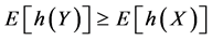 (1)
(1)
for all convex functions h. In terms of utility functions, (with  convex), this is the notion of second order stochastic dominance of X over Y (and Y is said to be more risky than X. [2] ).
Reflection certifies that the relationship (1) indeed yields a method for formalizing the intuitive notion that Y is more dispersed than X since, for random variable X and Y with the same means, (1) holds if and only if the mass of Y can be obtained from that of X by pushing the mass to the outside (dilating) while retaining the same center of gravity. This is the “mean preserving spread” notion used in financial analysis of return distributions [2] , the “Robin Hood transformation” used by economic researchers studying income distribution via Lorenz ordering [3] , and the “stop loss premium ordering” used by actuaries to rank order the riskiness of underwriting different hazards [4] .
In order to be able to rank distributions with differing means, it is useful to consider also the ordering defined by the inequalities
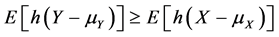 (2)
(2)
for all convex functions h for which the expectations in the above relationship (2) exist. Shaked [5] considered conditions that arise in applications which yield the inequalities (1) and (2). Rolski [6] , Whitt [1] and Brown [7] among others, studied the ordering defined by
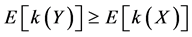 (3)
(3)
for all non-decreasing convex functions k such that the expectations in (3) exists. Roughly speaking, if (3) holds, then Y is “more dispersed” or is stochastically larger than X. The book by Gooaverts et al. [4] characterizes these orderings (and others) and discusses their implied interrationships in an insurance context.
Two of the most common measures of dispersion for a random variable X from a pre-specified value c are  and
and . (e.g., both are used in insurance and finance as risk measures). These two measures again have the form
 ![]() and can be used to define a total ordering on the space of distributions.
and can be used to define a total ordering on the space of distributions.
Unfortunately, in order to implement the above ordering criteria, it is necessary to know the entire probability distribution for the variables X and Y. Without such exact information, the expectation cannot be calculated in order to verify (1), (2) or (3). In many important practical problems, however, one only possesses partial information concerning the distribution of the variables under investigation. For example, in actuarial analysis, one may know the means (pure premium), the range of possible values for the variables (the policy limits and deductibles), and some information concerning the shape of the distributions (such as unimodality). In such situations (and with still further information such as higher moments), it is desirable to be able to assess the relative riskiness of one variable vis a vis the other. However, because the prescribed known information only incompletely determines the relevant distributions, it becomes necessary to compare the entire classes of distributions possessing the known characteristics. Accordingly, it is desirable to determine optimally tight upper and lower bounds on the expectation of the convex function of the variable under investigation where the supremum and infimum are taken over all random variables satisfying the given information constraints. This, then, produces a partial ordering on the space of probability distributions satisfying the informational constraints.
For a general function h(x) possessing nonnegative derivatives of one higher order than the number of known moments (e.g., ![]() or
or ![]() when only the mean is known, or
when only the mean is known, or ![]() with a known mean and variance), an explicit solution for the problem of obtaining the tightest possible bounds on
with a known mean and variance), an explicit solution for the problem of obtaining the tightest possible bounds on ![]() when X is unimodal with a known mode and a know range and finite set of moments was presented
when X is unimodal with a known mode and a know range and finite set of moments was presented
by Brockett and Cox [8] , and Brockett, Cox, and Witt [9] and used in Brockett and Kahane [10] and Brockett and Garven [11] . Their development was based on the theory of Chebychev systems of functions [12] coupled with Kemperman’s [13] “transformation of moments” technique.
This article begins by extending the arguments of Brockett and Cox [8] to a wider class of random variables (the so called alpha-unimodal or a-unimodal random variables). Then, to examine the more difficult case of
![]() which is not covered by the previously cited theorem, we use an approach based upon the results of Kemperman [14] on the geometry of the moment problem, which does not require differentiability.
which is not covered by the previously cited theorem, we use an approach based upon the results of Kemperman [14] on the geometry of the moment problem, which does not require differentiability.
2. Bounds on E[h(X)] for Arbitrarily Bounded X
We begin by restating a result from Brockett and Cox [8] . This Lemma gives the tightest possible bounds on expectations of functions of the type referred to above. We couple this with a yet unpublished result from Chang [15] to incorporate the situation when four moments are known.
Lemma 1: 1) Let ![]() be given and let h be a twice-differentiable function on
be given and let h be a twice-differentiable function on ![]() with
with ![]() for
for![]() . Then, for any random variable X with values in the interval
. Then, for any random variable X with values in the interval ![]() and mean
and mean![]() , we have the tight bounds
, we have the tight bounds ![]() where
where![]() .
.
2) Let ![]() and
and ![]() be given and let h be three times differentiable with
be given and let h be three times differentiable with ![]() for
for![]() . Then, for any random variable X with values in
. Then, for any random variable X with values in![]() , mean
, mean![]() , and variance
, and variance![]() , we have the tight bounds
, we have the tight bounds
![]()
where
![]()
and
![]()
3) Let![]() ,
, ![]() , and
, and ![]() be given, and let h be four times differentiable with
be given, and let h be four times differentiable with ![]() for
for![]() . Then, for any random variable X with values in
. Then, for any random variable X with values in![]() , mean
, mean![]() , variance
, variance![]() , and third moment
, and third moment![]() , we have the tight bounds,
, we have the tight bounds,
![]()
where
![]()
4) Let the 4-moment vector ![]() be given, and let h be five times differentiable with
be given, and let h be five times differentiable with ![]() for
for![]() . Then, for any random variable X with values in
. Then, for any random variable X with values in ![]() and the given four moments, we have the tight bounds,
and the given four moments, we have the tight bounds,
![]()
where
![]()
and where
![]()
Also,
![]()
where
![]()
Note that the bounds in the above theorem are optimal in the sense that there actually exist random variable ![]() and
and ![]() on
on ![]() with precisely the given set of moments for which the equality relation obtains,
with precisely the given set of moments for which the equality relation obtains,
namely that the distribution with the masses at the points specified within the argument of h(×) and with probability equal to the coefficient of h(×) on the sides of the two inequalities. Accordingly, the bounds cannot be improved without adding additional knowledge about the random variable X.
Before considering a-unimodal random variables, we note that a more general version of Lemma 1 can be proven in which the level of differentiability of h is decreased by one. In the case of a single moment ![]() being given, this means that we need not require h to be differentiable, but only that h be continuous and convex. This result, established for general numbers of moments by Chang [15] , is proven for the special case of convex functions in section 4, and follows from the fact that the function h can be uniformly approximated by a function with one larger derivative, and the fact that the bounding extreme measures do not depend on the actual function.
being given, this means that we need not require h to be differentiable, but only that h be continuous and convex. This result, established for general numbers of moments by Chang [15] , is proven for the special case of convex functions in section 4, and follows from the fact that the function h can be uniformly approximated by a function with one larger derivative, and the fact that the bounding extreme measures do not depend on the actual function.
3. Bounds on E[h(X)] When X Is Known to be Alpha-Unimodal
We now turn to the problem of obtaining bounds on the expectation when more is known about the distribution than just the moments. In particular, we generalize previous results to a general notion of distributional shape known as a-unimodality originally developed by Olshen and Savage [16] as a generalization of the usual notion of unimodality.
A random variable X is said to be a-unimodal with a-mode ![]() if it satisfies either (and hence both) of the following equivalent conditions
if it satisfies either (and hence both) of the following equivalent conditions
(i) X has the same distribution as ![]() where U and Y are independent random variables with U uniformly distributed on
where U and Y are independent random variables with U uniformly distributed on![]() .
.
(ii) ![]() is non-decreasing in
is non-decreasing in ![]() for every positive bounded measurable function g.
for every positive bounded measurable function g.
The case ![]() corresponds to the usual notion of unimodality and, in this situation, (i) is simply L. Shepp’s reformulation of Khinchine’s [17] characterization theorem for unimodality (cf., [18] page 158). The equivalence of (1) and (2) is due to Olshen and Savage [16] . From condition (ii) it is clear that if X is a-Unimodal, then
corresponds to the usual notion of unimodality and, in this situation, (i) is simply L. Shepp’s reformulation of Khinchine’s [17] characterization theorem for unimodality (cf., [18] page 158). The equivalence of (1) and (2) is due to Olshen and Savage [16] . From condition (ii) it is clear that if X is a-Unimodal, then
X is also b-unimodal for any![]() . Intuitively, in the case of an a-unimodal variable X with a-mode
. Intuitively, in the case of an a-unimodal variable X with a-mode![]() , this simply says that
, this simply says that ![]() for all x.
for all x.
Consider now a random variable X which is a-Unimodal on [a, b] with a-mode ![]() and which has given raw moments
and which has given raw moments![]() . By (i) we may write
. By (i) we may write ![]() where U and Y are independent random variables and U is uniformly distributed on [0,I]. The
where U and Y are independent random variables and U is uniformly distributed on [0,I]. The ![]() moment of
moment of ![]() is
is![]() , so the
, so the ![]() moment of Y is found by solving
moment of Y is found by solving
![]()
for![]() , which yields
, which yields![]() . The range of possible values for Y is
. The range of possible values for Y is![]() .
.
In many instances, it is more convenient to work with the central moments than the raw moments. In such situations the first three central moments of Y may be easily calculated in terms of the a-mode and central moments of X as below
![]()
In the case ![]() (ordinary unimodality), the above formulae reduce to the formulae of Brockett and Cox [8] for 1, 2, 3 moments given and allow the application of Lemma 1 to the random variable Y whenever the moments of X are known.
(ordinary unimodality), the above formulae reduce to the formulae of Brockett and Cox [8] for 1, 2, 3 moments given and allow the application of Lemma 1 to the random variable Y whenever the moments of X are known.
In order to emulate Kemperman’s “transfer of moment problems” technique for mixture variables, we proceed as follows. For![]() , consider the function g(y) obtained by calculating the expectation of h(X), conditional on
, consider the function g(y) obtained by calculating the expectation of h(X), conditional on![]() . This gives
. This gives
![]()
which, after the substitution![]() , can be reduced to
, can be reduced to
![]() ,
, ![]()
This is valid except perhaps at![]() . For
. For ![]() no change of variable is required and
no change of variable is required and![]() . For
. For![]() , this reduces to the formulae given in Brockett and Cox [8] [19] .
, this reduces to the formulae given in Brockett and Cox [8] [19] .
Note that![]() , so that h(X) and g(Y) have the same expectation. Accordingly, the problem of determining optimal bounds on E[h(X)] when X is a-unimodal with known moments and known a-mode can be transformed into the equivalent problem of obtaining bounds for
, so that h(X) and g(Y) have the same expectation. Accordingly, the problem of determining optimal bounds on E[h(X)] when X is a-unimodal with known moments and known a-mode can be transformed into the equivalent problem of obtaining bounds for![]() .
.
When the only information about Y is its range and a known set of moments calculated from the moments of X via the above-derived formulae. Applying Lemma 1 to the variable Y and function g then produces optimal bounds for E[g(Y)] and hence E[h(X)]. This is summarized in the following theorem.
Theorem 1. Let X be an a-unimodal random variable on [a, b] with mean![]() , variance
, variance ![]() third central moment
third central moment![]() , and a-mode
, and a-mode![]() . Let g denote the function
. Let g denote the function
![]()
![]()
and![]() .
.
1) If ![]() is given and h is twice differentiable on [a, b] with
is given and h is twice differentiable on [a, b] with ![]() for
for![]() . Then we have tight bounds
. Then we have tight bounds
![]()
where ![]()
2) If ![]() and
and ![]() are given and h is three times differentiable with
are given and h is three times differentiable with ![]() for
for![]() . Then, we have the tight bounds
. Then, we have the tight bounds
![]()
where
![]()
and
![]()
3) If![]() ,
, ![]() and
and ![]() are given and h is four times differentiable with
are given and h is four times differentiable with ![]() for
for![]() . Then we have the tight bounds
. Then we have the tight bounds
![]()
where
![]()
![]()
![]()
![]()
![]()
![]()
and where![]() , and
, and ![]() are given in terms of
are given in terms of ![]() and
and ![]() according to the formulae given in the previous section.
according to the formulae given in the previous section.
4) Let the 4-moment vector ![]() be given, and let h be five times differentiable with
be given, and let h be five times differentiable with ![]() for
for![]() . Then, for any random variable X with values in
. Then, for any random variable X with values in ![]() and the given four moments, we have the tight bounds,
and the given four moments, we have the tight bounds,
![]()
where
![]()
and where
![]()
Also,
![]()
where
![]()
Note that the derived function g(y) on ![]() also inherits the nonnegative
also inherits the nonnegative ![]() derivative properties of h on [a, b]. Accordingly, Theorem 1 follows from Lemma 1 applied to the function g and the random variable Y due to the fact that
derivative properties of h on [a, b]. Accordingly, Theorem 1 follows from Lemma 1 applied to the function g and the random variable Y due to the fact that![]() . A numerical illustration of this theorem is given in Table
. A numerical illustration of this theorem is given in Table
1 for the function![]() , using the given support a = 0, b = 10 and the moment knowledge
, using the given support a = 0, b = 10 and the moment knowledge
![]() and mode = 5. This is done first with only support and moment knowledge, and
and mode = 5. This is done first with only support and moment knowledge, and
![]()
Table 1. Bounds on the expectation ![]() of an alpha-unimodal random variable with different moment knowledge, alpha = 2.
of an alpha-unimodal random variable with different moment knowledge, alpha = 2.
then with this knowledge plus the knowledge that the random variable in question is a-unimodal with![]() . As can be seen, at each given level of moment knowledge, the additional knowledge of a-unimodality improves the optimal bounds.
. As can be seen, at each given level of moment knowledge, the additional knowledge of a-unimodality improves the optimal bounds.
Note that in each case the permissible range of values with known unimodal situation is smaller than when unimodality is not known, and that the “indeterminacy” range decreases (sometimes dramatically) as more moments and unimodality are added.
4. Bounds on ![]() and
and ![]() with X Being Alpha-Unimodal
with X Being Alpha-Unimodal
As mentioned previously, there are certain functions h which are particularly important as measures of risk in applications. One such function is ![]() on the interval [a, b]. For this function, we calculate g(y) as follows:
on the interval [a, b]. For this function, we calculate g(y) as follows:
![]()
![]() , and
, and![]() .
.
According to Theorem 1, the best bounds on this squared distance measure given the partial stochastic information can be explicitly obtained. We summarized the result as follows.
Theorem 2. Let X be an a-unimodal random variable on [a, b] with mean ![]() and a-mode
and a-mode![]() . Then the second moment of X about c is optimally bounded as follows:
. Then the second moment of X about c is optimally bounded as follows:
![]()
Proof: From Theorem 1 the optimal bounds are
![]()
where ![]() and g is the quadratic polynomial
and g is the quadratic polynomial
![]()
The lower bound is g(E[Y]) which is calculated as follows:
![]()
The upper bound is E[g(Y)] which is
![]()
Now use the definition of p to find
![]()
which completes the proof.
Corollary 1. Let X be an a-unimodal random variable on [0, 1] with mean ![]() and a-mode
and a-mode![]() . Then the variance of X is optimally bounded as follows:
. Then the variance of X is optimally bounded as follows:
![]()
Proof: This follows directly from Theorem 2 by setting a = 0, b = 1, and![]() . (We note that the upper bound in Corollary 1 was also obtained by Dharmadhikari and Joag-Dev [20] by a completely different argument.)
. (We note that the upper bound in Corollary 1 was also obtained by Dharmadhikari and Joag-Dev [20] by a completely different argument.)
We now turn to the analogue of the situation occurring in symmetric unimodal situations wherein the mean and mode coincide.
Corollary 2. Let X be a-unimodal on [a, b] with mean ![]() and a-mode
and a-mode![]() . Then the second moment of X about c is optimally bounded as follows:
. Then the second moment of X about c is optimally bounded as follows:
![]()
In particular, if X is a-unimodal on [0, 1] with![]() , then the upper bound becomes
, then the upper bound becomes ![]() and the variance of X is optimally bounded by
and the variance of X is optimally bounded by![]() . The upper bound on the variance equals
. The upper bound on the variance equals ![]() in the ordinary unimodal case (
in the ordinary unimodal case (![]() ).
).
Proof: This follows by assigning the values![]() , and
, and ![]() in Theorem 1.
in Theorem 1.
Another function of importance in risk applications is the function![]() . In order to apply Theorem 1 to this function we must calculate
. In order to apply Theorem 1 to this function we must calculate
![]()
![]() ,
,
except that![]() . In the case at hand, we find that
. In the case at hand, we find that
![]()
For values of c in the range![]() , we find that
, we find that
![]()
The case of c
![]() , for
, for ![]()
While for c>b, we have
![]() , for
, for ![]()
Since ![]() is integrable and convex, g(y) is also convex.
is integrable and convex, g(y) is also convex.
The lack of differentiability of h and g makes the routine application of Theorem 1 impossible. However a technique of Kemperman [13] [14] can be used to overcome these technical difficulties. To this end we briefly describe Kemperman’s approach to moment problems.
Let X denote a random variable on [a, b] with specified moments ![]() for
for![]() , and assume the function
, and assume the function ![]() is continuous (slightly weaker continuity conditions are allowed by Kemperman). We denote by
is continuous (slightly weaker continuity conditions are allowed by Kemperman). We denote by ![]() the set of all “admissible” distributions F for X, i.e., those satisfying
the set of all “admissible” distributions F for X, i.e., those satisfying ![]() and
and
![]() , for
, for![]() ,
,
where ![]() represents the vector of moments which are assumed to be known (given). The upper and lower bounds on the expected value of a function h(x) subject to X having the prescribed set of moments
represents the vector of moments which are assumed to be known (given). The upper and lower bounds on the expected value of a function h(x) subject to X having the prescribed set of moments ![]() are denoted
are denoted ![]() and
and ![]() respectively, i.e.,
respectively, i.e.,
![]()
and
![]() .
.
Kemperman defines an upper contact polynomial relative to the specified moment problem for ![]() to be a polynomial
to be a polynomial ![]() of degree n (equal to the number of specified moments) for which
of degree n (equal to the number of specified moments) for which ![]() for all x in [a, b]. The corresponding contact set is Z(q) = {x|
for all x in [a, b]. The corresponding contact set is Z(q) = {x|![]()
and q(x) = h(x)}. Lower contact polynomials and the corresponding contact sets are defined analogously as lying
below and touching h. Note that if there is an admissible distribution ![]() for which
for which ![]() (i.e., there is a distribution with the specified moments
(i.e., there is a distribution with the specified moments ![]() which has its support on the contact set Z(q)), then
which has its support on the contact set Z(q)), then ![]() provides the numerical upper value to the upper limit of the moment problem. To see this note that
provides the numerical upper value to the upper limit of the moment problem. To see this note that
![]()
Moreover, for any other distribution G in ![]() the expected value of h satisfies
the expected value of h satisfies
![]() ,
,
so ![]() indeed provides the upper bound
indeed provides the upper bound![]() .
.
One of the important results of Kemperman is that for any continuous function h there is always a contact polynomial q and distribution ![]() in
in ![]() concentrated on Z(q). Moreover, a similar situation can also be seen to apply to the problem of obtaining a lower bound on the expected value of a function h (i.e., for the lower part of the moment problem).
concentrated on Z(q). Moreover, a similar situation can also be seen to apply to the problem of obtaining a lower bound on the expected value of a function h (i.e., for the lower part of the moment problem).
As an illustration of Kemperman’s theorems we generalize the previously stated result to the case where h is not differentiable (so does not satisfy![]() ) but is convex. The function
) but is convex. The function ![]() is an example of such a function. It arises in insurance as the negative of the stop loss premium function with deductible level c and also occurs in the financial theory of option pricing. The function
is an example of such a function. It arises in insurance as the negative of the stop loss premium function with deductible level c and also occurs in the financial theory of option pricing. The function ![]() is another such function.
is another such function.
Theorem 3. Let X be a random variable on [a, b] with mean![]() , and let h be a continuous convex function. Then we have tight bounds
, and let h be a continuous convex function. Then we have tight bounds
![]()
where![]() .
.
Proof: Using Kemperman’s results we know that
![]() ,
,
where ![]() is a lower contact polynomial and
is a lower contact polynomial and ![]() is a distribution concentrated on Z(q). The graph of q(x) is a straight line and the graph of h is convex up so the contact set is either a point or an interval. If Z(q) = {z} is a single point, then
is a distribution concentrated on Z(q). The graph of q(x) is a straight line and the graph of h is convex up so the contact set is either a point or an interval. If Z(q) = {z} is a single point, then ![]() is a one point distribution with mean
is a one point distribution with mean![]() , so
, so ![]() .
.
Similarly, if the contact set is an interval![]() , then h is linear on Z(q) and hence
, then h is linear on Z(q) and hence
![]()
in this case as well. This shows that ![]() is the lower bound in either case. For the upper bound, we have
is the lower bound in either case. For the upper bound, we have ![]() where
where ![]() is concentrated on Z(q), and again q is a linear polynomial whose
is concentrated on Z(q), and again q is a linear polynomial whose
graph now lies above the graph of h. Because the graph of h is convex, the contact set is exactly the two end
points, Z(q) = {a, b} so the extremal measure ![]() is concentrated on the two points {a, b}. Thus
is concentrated on the two points {a, b}. Thus ![]() . Since
. Since ![]() the mean is
the mean is![]() , so the unknown p can be determined from the moment equation
, so the unknown p can be determined from the moment equation![]() . i.e.,
. i.e.,![]() . This establishes the upper bound term in the theorem, and provides the prototype method for constructing optimal bounds in the general situation in which an arbitrary number of moments are known.
. This establishes the upper bound term in the theorem, and provides the prototype method for constructing optimal bounds in the general situation in which an arbitrary number of moments are known.
Using Theorem 3, we may find the best bounds on ![]() in the same manner as before. We summarize this result as follows.
in the same manner as before. We summarize this result as follows.
Theorem 4. Let X be an a-Unimodal random variable on [a, b] with mean ![]() and a-mode
and a-mode![]() . The expected absolute deviation of X from c is optimally bounded as follows:
. The expected absolute deviation of X from c is optimally bounded as follows:
![]()
where
![]() ,
, ![]() ,
,
and g(y) is defined as follows: For c in the range![]() ,
,
![]()
while for c < a,
![]() for
for![]() ,
,
and for c > b,
![]() for
for![]() .
.
Some simple examples follow immediately.
Corollary 3. Let X be a-unimodal on [0, 1] with a-mode ![]() and mean
and mean![]() . The absolute deviation from
. The absolute deviation from ![]() is optimally bounded as follows:
is optimally bounded as follows:
![]()
For the special case![]() ,
,
![]() ,
,
while in the ordinary unimodal case (![]() ),
),
![]()
Proof: Applying Theorem 4 with a = 0, b = 1, and![]() , yields
, yields ![]() for
for![]() . The lower bound is
. The lower bound is![]() . The upper bound is
. The upper bound is
![]()
The special cases for ![]() and
and ![]() can now be obtained by substitution.
can now be obtained by substitution.
5. Application: Assessing the Probability of Ruin Using Incomplete Loss Distribution Information
Here, we only briefly sketch the collective risk model from actuarial science since the development is quite complete in Bowers, et al. [21] . The cash surplus at time t is defined to be
![]()
Here ![]() is the initial surplus, c is the rate at which premiums are credited to the fund in dollars per year, and S is the stochastic claims process:
is the initial surplus, c is the rate at which premiums are credited to the fund in dollars per year, and S is the stochastic claims process:
![]()
where ![]() is a Poisson process with parameter
is a Poisson process with parameter ![]() and
and ![]() are the independent and identically distributed loss variables. Ruin is said to occur if
are the independent and identically distributed loss variables. Ruin is said to occur if![]() , that is, if the cash surplus falls below zero.
, that is, if the cash surplus falls below zero.
We are interested here in determining the probability that there is eventual ruin as a function of the initial reserve![]() . Let us denote this probability by
. Let us denote this probability by![]() . The main theorem of chapter 12 of Bowers et al. [21] is
. The main theorem of chapter 12 of Bowers et al. [21] is
![]()
where ![]() is the time of ruin, and R is the so-called adjustment coefficient which
is the time of ruin, and R is the so-called adjustment coefficient which
depends upon three things: the distribution of the losses, X, the frequency with which losses occur, ![]() , and the load factor
, and the load factor![]() , which was used for setting the premium. By definition the adjustment coefficient is the smallest positive solution to the equation
, which was used for setting the premium. By definition the adjustment coefficient is the smallest positive solution to the equation
![]()
where X is a random variable having the common distribution of the losses, ![]() , and
, and ![]() is the premium charged, and
is the premium charged, and ![]() is the moment generation function for X. There is a unique positive solution R to the above equation provided only that
is the moment generation function for X. There is a unique positive solution R to the above equation provided only that![]() .
.
Assuming now that we have only partial knowledge about the loss variable X, we do not know ![]() and hence cannot directly solve for
and hence cannot directly solve for![]() . We can, however, use the partial information about the moments of X to determine bounding curves on
. We can, however, use the partial information about the moments of X to determine bounding curves on![]() . We have from Lemma 1 with
. We have from Lemma 1 with ![]() for
for![]() ,
,
![]()
where ![]() and
and ![]() denote the moment generating functions of the lower and upper probability distribution occurring in the inequalities of the Lemma 1, for the moments of the loss distribution which we have. Thus if
denote the moment generating functions of the lower and upper probability distribution occurring in the inequalities of the Lemma 1, for the moments of the loss distribution which we have. Thus if ![]() and
and![]() ,
, ![]() and
and ![]() are known, then one can numerically solve for
are known, then one can numerically solve for ![]() and
and![]() , the adjustment coefficients corresponding to the upper and lower bounding distribution with the given moments. For all
, the adjustment coefficients corresponding to the upper and lower bounding distribution with the given moments. For all ![]() the curves satisfy
the curves satisfy ![]() since the extremal measures
since the extremal measures ![]() and
and ![]() do not depend upon r in
do not depend upon r in![]() . At
. At![]() , the functions
, the functions ![]() and
and ![]() are equal to 1 and have slopes of
are equal to 1 and have slopes of![]() . Since
. Since![]() , the graph of
, the graph of ![]() has a slope which is strictly greater than
has a slope which is strictly greater than![]() . As shown in Brockett and Cox [19] , the line
. As shown in Brockett and Cox [19] , the line ![]() intersects these curves exactly twice, once
intersects these curves exactly twice, once
at zero and once at a positive value. The intersections for the positive values are precisely in order![]() ,
, ![]() and
and ![]() from left to right as shown in Figure 1. Hence the corresponding adjustment coefficients must satisfy
from left to right as shown in Figure 1. Hence the corresponding adjustment coefficients must satisfy ![]() as pictured in the following chart.
as pictured in the following chart.
From the above formula for ![]() we easily obtain the bounds on the ruin probability, namely
we easily obtain the bounds on the ruin probability, namely
![]() . The RHS inequality is due to
. The RHS inequality is due to ![]() and
and![]() ; the LHS inequality comes from
; the LHS inequality comes from ![]() hence
hence![]() . Now given the moments of the loss distribution, X, we may determine the upper and lower extremal probability distributions as given in Lemma 1, that is, let
. Now given the moments of the loss distribution, X, we may determine the upper and lower extremal probability distributions as given in Lemma 1, that is, let ![]() in Lemma 1, and hence we can solve numerically for
in Lemma 1, and hence we can solve numerically for ![]() and
and![]() , from the
, from the
![]()
Figure 1. Bounds on the adjustment coefficient using partial information.
bounds ![]() and
and![]() . These values are just the adjustment coefficients corresponding to the extremal distributions assuming
. These values are just the adjustment coefficients corresponding to the extremal distributions assuming ![]() and
and ![]() respectively are the distribution for X.
respectively are the distribution for X.
We find the following bounds on the ruin probability using partial information:
![]()
As an example, consider a group medical insurance policy which covers from the first dollar of loss up to a maximum of $5000. Assume that moments![]() ,
, ![]() , and
, and ![]() of claim size are known and the rate of frequency of claims,
of claim size are known and the rate of frequency of claims, ![]() , is also known. We will approximate R, the adjustment coefficient, using the numerical values
, is also known. We will approximate R, the adjustment coefficient, using the numerical values
![]()
![]() , and the mean
, and the mean ![]() Next we will include the information that
Next we will include the information that ![]() into the calculation, the skewness measure
into the calculation, the skewness measure![]() , and the Kurtosis measure
, and the Kurtosis measure![]() . It should be em-
. It should be em-
phasized that the bounds on R are tight in the sense that both equalities are possible. These bounds cannot be improved without specifically obtaining more information about X.
Table 2 presents the numerical results. The values of ![]() can be used to give upper bounds on
can be used to give upper bounds on![]() , the ruin probability, because
, the ruin probability, because ![]()
6. Improvements in the Bounds When the Random Variables Are Known to Be Alpha-Unimodal
Often more is known about the return distribution than just the first few central moments. For example, the distribution of X is frequently known to be a-unimodal, or just plainly unimodal. In this section, we show how to use this information to improve the Chebychev system bounds. The starting point for incorporating unimodality into the bounds is the results of the previous sections, showing that if a random variable X is a-unimodal with
a-mode![]() , then
, then ![]() is a-unimodal about 0. According to Theorem 1,
is a-unimodal about 0. According to Theorem 1,![]() .
.
The critical impact of the loss distribution X on the probability of ruin ![]() with initial reserve u came through the adjustment coefficient R. This was the point of intersection of the moment generating function
with initial reserve u came through the adjustment coefficient R. This was the point of intersection of the moment generating function ![]() with the line
with the line![]() . If we know the first few moments of X and its mode m, then we
. If we know the first few moments of X and its mode m, then we
![]()
Table 2. Bounds upon the adjustment coefficient using only moment information.
*Notice particularly how quickly the width of the interval of indeterminacy decreases as more moments are included.
transform the moment problems involved in the calculation of ![]() as follows:
as follows:
![]()
where ![]() based on Theorem 1. The moment information of auxiliary variable y can be obtained from above sections. We now use Theorem 1 to bound
based on Theorem 1. The moment information of auxiliary variable y can be obtained from above sections. We now use Theorem 1 to bound![]() . Once we have determined the extremal measures of
. Once we have determined the extremal measures of ![]() and
and![]() , we find their adjustment coefficients by finding their intersections with the line
, we find their adjustment coefficients by finding their intersections with the line![]() . To be explicit, we find the intersection of the curves
. To be explicit, we find the intersection of the curves
![]()
and
![]()
with the line ![]() in order to find the bounds on the adjustment coefficient. This is shown graphically in Figure 2.
in order to find the bounds on the adjustment coefficient. This is shown graphically in Figure 2.
As a numerical illustration, we return to the example of last section. Here we shall assume additionally that the loss distribution is known to be a-unimodal with the most likely or modal value![]() . Our best bounds on the adjustment coefficient R are now obtained by translating the original loss variable moments from X to Y, via the equations above, then using Theorem 1 to find the explicit formulas for the extremal measures for Y, and
. Our best bounds on the adjustment coefficient R are now obtained by translating the original loss variable moments from X to Y, via the equations above, then using Theorem 1 to find the explicit formulas for the extremal measures for Y, and
then calculating the bounds for![]() . The corresponding numerical values for the adjustment coefficient R
. The corresponding numerical values for the adjustment coefficient R
are given in Table 3. Note that in each situation, the bounds obtained by using the unimodality assumption are
![]()
Figure 2.The best bounding curves for ![]() given unimodality, and their corresponding bounds upon the adjustment coefficient.
given unimodality, and their corresponding bounds upon the adjustment coefficient.
![]()
Table 3. Bounds on the adjustment coefficient based on moments and unimodality of the loss variable*.
*If the loss is known to be alpha-unimodal with alpha = 1.
strictly tighter than those obtained without unimodality. These bounds cannot be improved without further information about the loss variable X.
The upper and lower bounds on the adjustment coefficient can be translated into estimates for the initial reserve u needed to insure a probability of eventual ruin of a pre-specified size. The calculations involving unimodality will yield more accurate estimates for this initial reserve than would the calculations without unimodality information.
7. Conclusion
The desire to stochastically order two random variables X and Y with respect to “dispersion” or “variability” occurs in several application areas such as nonparametric statistics, queuing theory, financial economics, and actuarial science. In many applications, however, the information about the distributions involved is not complete. One may know only the general range of values, the first few moments, and perhaps that the shape is unimodal. In such circumstances the explicit calculation of the relevant expectations needed to implement the traditional stochastic ordering techniques impossible, and it is necessary to find bounds on these expectations instead. This paper derives tight upper and lower bounds on the expectations of functions of incompletely determined distributions, and applies these results to the class of a-unimodal variables (a generalization which includes ordinary unimodality as a special case). Optimal bounds on the variance and absolute deviation of a-unimodal random variables are presented as illustrations of the technique. Such bounds may also be useful for calculations in PERT type networks in which the individual completion time distributions are not exactly known, but partial information concerning the properties of the distributions can be deducted.
References