Contrast Optimization for an Animal Model of Prostate Cancer MRI at 3T ()
Received 10 March 2016; accepted 26 April 2016; published 29 April 2016

1. Introduction
Magnetic Resonance Imaging (MRI) has high spatial resolution and the best soft tissue contrast among in vivo imaging modalities [1] , [2] . However, contrast to noise ratio (CNR) of some cancerous tissues is still often insufficient for accurate diagnosis [3] . Normal and diseased tissues are difficult to differentiate in standard T1 or T2-weighted MRI, [4] in particular when tissues have similar relaxation times, such as prostate tumours and surrounding tissue [1] , [5] . This poor differentiation between healthy and malignant tissue often leads to overtreatment degrading future quality of life of cancer patients [6] . To rectify this problem, contrast agents are used. However their multiple application can lead to unwanted side effects [7] . Therefore, the purpose of this work was to find out the optimal echo time (TE) that provides the maximum CNR using a spin-echo pulse sequence for MRI of prostate cancer at 3T.
MR signal of a tissue is a function of its spin density and relaxation times [8] . It can be controlled by the pulse sequence parameters, such as echo time (TE), repetition time (TR) or flip angle of a radiofrequency (rf) pulse. As the contrast depends on a difference in signals generated by two samples it can be maximized by selecting optimum parameters of the pulse sequence.
Optimization of MRI pulse sequence parameters has been a field of interest since the beginning of MRI [9] - [11] . The presented solution is different from previous methods by providing a simplistic but effective solution to obtain the maximum CNR between tissues, specifically for prostate cancer. An early study used a method known as Eigen image Filtering to optimize MRI protocols and pulse sequence parameters. This study was able to reduce imaging time for eigen image filtering of brain studies by up to 75% however approximation of tissue parameters from literature was needed, otherwise further tissue parametrization would be needed [9] . Another study used sequence simulations to predict optimal parameters for imaging, however simulated images failed to match the corresponding measured image in areas where tissues or substances moved during the course of measurement. The phenomena of flow could not be feasibly incorporated into the equations [10] . A study in 1987 compared the ability if different T1, T2 and proton density (PD) weighted imaging would increase or decrease CNR for hepatic lesions among patients. They concluded that although short-TE T1-weighted pulse sequences with multiple excitations has the best signal to noise ratio and anatomic resolution at 0.6T, their described technique is limited by relatively inferior contrast discrimination and artifact suppression at 1.5T resulting in a necessary change in imaging strategy when performing hepatic MR imaging at 1.5T [11] . Specifically, for prostate cancer, many studies have incorporated the use of diffusion weighted imaging (DWI) and apparent diffusion coefficient maps (ADC) to increase detection of prostate cancer. However, these methods are only viable with MRI above 1.5T as lower fields do not have the SNR required to create quality DWI and ADC maps [4] , [12] . These studies have increased the differentiability of prostate cancer from healthy prostate tissue but require more intensive image processing. Our work follows a similar derivation proposed in [8] but used a solution for spin echo imaging instead of gradient echo and we have optimized CNR for tissues with small differences in T2. Furthermore, the method does not require absolute values of proton density. Instead we worked with relative values of proton densities between tissues with a method suggested by [13] . A similar method using derivatives is used to determine the concentration of contrast agent needed to optimize the Ernst angle in T1-weighted spoiled gradient echo imaging [14] and optimal TE to determine maximum SNRefficiency for MR-guided interventional procedures [15] .
The solution presented in this work maximizes CNR by optimizing TE in the spin-echo pulse sequence. Using a formula for MR signal obtained with the spin-echo pulse sequence and knowing T2s of the samples we calculated TEmax that provided the maximum CNR for in vitro phantoms and in vivo for prostate and surrounding tissues at 3T.
2. Methods
For the calculations of CNR we used an equation providing a relationship between CNR and pulse parameters. We have assumed T2 relaxation times are known and T1relaxation can be neglected. Nine samples with different T2 relaxation times were made using different water concentrations of superparamagnetic iron oxide (SPIO). CNR as a function of TE was calculated for all sample pairs. The theoretical results were compared to the MRI experiments in vitro and in vivo using the animal model of prostate cancer at 3T.
2.1. Theory
Contrast in MR imaging can be defined as the difference in signals from two samples [8] , [16] , [17] .
 (1)
(1)
where SNR1 and SNR2 are the signal to noise ratios of two samples.
The MR signals from two samples (S1 and S2) using spin-echo pulse sequence can be described as: [8] , [16]
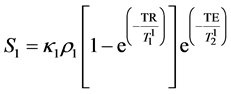 (2)
(2)
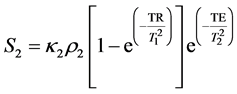 (3)
(3)
where κ1, κ2 are the proportionality constants, ρ1, ρ2 are the spin densities,  ,
,  and
and ,
,  are the longi-
tudinal and transversal relaxation times of the sample 1 and 2 respectively; TR is the repetition time and TE is the echo time. Each signal for samples is divided by the standard deviation, σ, in the image to obtain SNR.
Subtracting (2) from (3) we obtain CNR for the samples 1 and 2:
 (4)
(4)
Assuming TR is sufficiently long ( ), and taking the derivative of Equation (4) with respect to TE, the maximum for CNR can be obtained at:
 (5)
(5)
As seen from Equation (5), TEmax depends only on the T2 relaxation times of the samples thus it can be calculated to provide the maximum CNR if only T2s are known.
The results of the calculation for different samples pairs are presented in Table 2 where each sample has a T2 value and each sample pair has a corresponding TEmax.
2.2. In Vitro Experiments
2.2.1. Sample Preparation in Vitro
Molday ION Rhodamine Carboxyl, a commonly used SPIO, (MIRB, Cat #: CL-50Q02-6C-50, BioPAL, Inc, Worcester, MA, USA) was diluted in de-ionized water to prepare nine samples (0.0019, 0.0022, 0.0029, 0.0042, 0.0061, 0.0071, 0.0083, 0.0121, and 0.0263 μg/μL).The samples were placed in standard 5-mm NMR tubes (Wilmad NMR tubes, Cat#: Z566411-5EA, Sigma Aldrich, St. Louis, MO, USA) and arranged in a grid pattern to allow simultaneous imaging of all samples.
2.2.2. MR Imaging and T2 Calculations
MR imaging was performed using a 3T MRI scanner (Achieva, Philips, The Netherlands). Data was acquired using an 8-channel head RF coil. The spin echo pulse sequence with the following parameters was used: 32 echoes, ΔTE = 20 ms, TR = 5000 ms, FOV = 100 mm × 100 mm, 3 mm slice thickness, 224 × 224 matrix size, NEX = 4. The images were transferred to an external workstation and processed with custom MATLAB scripts (MATLAB and Statistics Toolbox Release R2012a, The MathWorks, Inc., Natick, Massachusetts, United States). A region of interest (ROI) was automatically selected for each sample as a circular area within the sample for in vitro data. The ROI was determined by a mask with a pre-determined threshold in order to make ROIs determination quick and without human error.Single exponential fitting of the echo train was used to calculate TTs according to the formula:
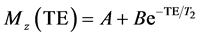 (6)
(6)
where Mz is the signal intensity at the echo time TE; A, B and T2 are the fitting parameters.8
2.3. In Vitro Experiments
2.3.1. Animal Model
To induce prostate tumours, 5 × 10⁶ LNcaP cells suspended in 100 μL of PBS were subcutaneously injected in the flank of 8 male athymic nude mice (Charles River, Wilmington, MA, USA). The mice were anesthetized with isoflurane (Baxter International Inc., Deerfield, IL, USA) during MR imaging and euthanized immediately after.MR imaging of mice was performed once tumours reached a diameter of 5mmusing calipers according to our approved protocol (Lakehead University Animal Care Committee).
2.3.2. MR Imaging and T2 Calculations
Data was acquired using the MESE pulse sequence with an 8-channel wrist RF coil with the following parameters: 30 echoes, ΔTE = 8 ms, TR = 1396 ms, FOV = 240 mm × 240 mm, slice thickness = 3 mm, 156 × 156 matrix, NEX = 4. Processing was performed similarly to in vitro experiments but ROIs were manually determined for the tumour, muscle, and kidney.
2.4. CNR Calculations
CNR was calculated from the MESE image sets for various echo times. Signal intensity of each sample was normalized to the signal intensity of the first echo for each sample for in vitro data and we assumed κ1ρ1 = κ2ρ2. For CNR calculations in vivo, ρ and κ constants were found using the method described by Tofts et al. [13] where the values of each κ, ρ for each sample were extrapolated putting TE = 0 in Equation (2) and (3) for MESE images. The method used yields a relative κ, ρ for each tissue compared to other tissues. This is then used to find the ratio of κ, ρ between samples which is then used in Equation (5).
A series of CNR curves as a function of TE were calculated and drawn for all the sample pairs using Equation (5) and cross correlation was used to determine the similarity between the theoretical and the experimental CNR curves.
In order to compare the theoretical and the experimental results of CNR, two parameters were defined. The first parameter  described deviation between theoretical and experimental echo time for maximum CNR and was defined as
 (7)
(7)
where TEExp is the experimental TE value at which the maximum CNR occurred and TETh is the theoretical TE value at which the maximum CNR was predicted to occur.
The second parameter  indicated differences in predictions from theoretical and experimental results of measured CNR
 (8)
(8)
where ![]() is the maximum CNR observed experimentally. TETh is the theoretical calculated value of TE (Equation 6) at which CNR is maximum.
is the maximum CNR observed experimentally. TETh is the theoretical calculated value of TE (Equation 6) at which CNR is maximum.
3. Results
3.1. In Vitro
T2-weighted MR image of the 9 samples used for analysis is shown in Figure 1. Their calculated T2 values are shown in Table 1.
The calculated TE values providing maximum CNR for each sample pair are shown in Table 2.
Figure 2 shows four examples of CNR as a function of TE for different sample pairs; T2 = 96 and 26 ms, 193 and 53 ms, 193 and 123 ms, and 679 and 86 ms. The corresponding TEmax values are 46.6, 60.2, 133.4 and 146.6 ms respectively.
The theoretical curves for these samples are superimposed on the experimental results. The mean cross correlation value between the experimental and theoretical curves was r = 0.98 ± 0.02.
The mean percent difference between the theoretical and experimental TEs at which the maximum (![]() ) occurred was 5.1% ± 5.3%. The mean percent difference for maximum CNR (
) occurred was 5.1% ± 5.3%. The mean percent difference for maximum CNR (![]() ) was.32% ± 0.71%.
) was.32% ± 0.71%.
![]()
Figure 1. T2-weighted (TE = 40 ms) in vitro MR image. Longest T2 is at the top left and the shortest T2 is at the bottom right.
![]() (a) (b)
(a) (b)![]() (c) (d)
(c) (d)
Figure 2. CNR as a function of TE based on theoretical calculations and experimental data: (a) sample 6 (T2 = 96 ms) vs sample 9 (T2 = 26 ms); (b) sample 4 (T2 = 193 ms) vs sample 8 (T2 = 53 ms); (c) sample 4 (T2 = 193 ms) vs sample 5 (T2 = 123 ms); and (d) sample 1 (T2 = 679 ms) vs sample 7 (T2 = 86 ms).
![]()
Table 1. T2 values of in vitro samples.
![]()
Table 2. TE values providing maximum CNR for two samples. The top row and the left columns indicate the T2 values of the sample pair. For example: maximum CNR for a sample pair with T2 123 ms and 53 ms is obtained at a TE of 51.2 ms.
3.2. In Vivo
Figure 3 shows sagittal MR images of the mouse torso at TE values of 56 ms and 96 ms. T2 of the tumor and normal tissue was found to be 55.8 ± 8.8 ms and 32.9 ± 2.4 ms for all 8 mice respectively. Based on the calculations maximum CNR between muscle and tumour tissue was found to occur at 55.2 ms. Typical T2-weighted images of human prostate cancer use an echo time of around 96 ms [12] . The images at TE = 56 ms (Figure 3(b)) showed CNR increase of 125% compared to an image at TE = 96 ms (Figure 3(a)). Mean correlation values, ![]() and
and ![]() were 0.94 ± 0.01, 21.2% ± 19.4% and 7.83% ± 7.45% respectively.
were 0.94 ± 0.01, 21.2% ± 19.4% and 7.83% ± 7.45% respectively.
Figure 4 shows CNR as a function of TE for muscle, kidney and tumour tissue. A visible CNR maximum appears between tumour and muscle at TE of 56 ms. In vivo experimental curves had high cross correlation values of r = 0.98 ± 0.01 and were able to attain maximum CNR based on predictions showing good agreement between the theory and the experiment.
4. Discussion
The results have shown that it was possible to maximize CNR by selecting the proper TE for SE pulse sequences when T2 relaxation times of the samples are known. The experiments showed that the theory indeed provides the parameters allowing maximum CNR. The cross correlation function showed the theoretical values closely emulated experimental data.
For in vitro calculations we assumed![]() . This is only valid if we consider the proton density to be the same for each sample. In these experiments it was deemed valid since all the samples were contained distilled water with only negligible amounts of MIRB added.
. This is only valid if we consider the proton density to be the same for each sample. In these experiments it was deemed valid since all the samples were contained distilled water with only negligible amounts of MIRB added.
As it can be seen in Figure 4 the predicted maximum of CNR between the cancerous tissue and the kidney is at TE = 131.6 ms. However, higher CNR values are also observed for TEs shorter than ~50 ms. This may be caused by differences in proton densities or differences in short T2 component. In this case where tissues have large differences in proton densities, acquiring a proton density image at short TE could result in an image of higher CNR. This may require the use of very short TE which may not be feasible with some current MRI hardware [17] .
One deficiency of Equation (5) is the possibility of resulting in a negative value of the optimal TE. In some cases, where T2 values are close and there are large differences in proton density, assuming κ is the same, the equation results in a negative TE value. For example, if the T2 values are 32.9 and 55.8 ms for tumour and muscle tissue respectively, and ρ1 is half of ρ2, the resulting optimal TEmax is −13.2 ms. This result has no physical meaning so for these cases choosing the smallest TE value possible should result in the best possible CNR.
The experimental values showed CNR can be maximized between prostate cancer and muscle tissues when their T2 values differed by about 15 ms. However, in clinical practice, the difference in MRI parameters between malignant prostate cancer and healthy prostate tissue is much lower [4] . Therefore although the proposed me-
![]() (a) (b)
(a) (b)
Figure 3. In vivo MR images of a mouse at (a) TE = 96 ms and (b) TE = 56 ms. Region of interests used for CNR calculations tumour, muscle, and kidney as red (―), blue (--) and green (…) respectively. By using predicted TEmax; (b) has an 125% CNR compared to (a).
![]()
Figure 4. In vivo experimental and theoretical CNRas a function of TE comapring tumour with muscle and kidney.
thod has the ability to maximize CNR between healthy and malignant tissue, further work with patients is needed to investigate the differentiation of healthy prostate tissue from malignant tissue in humans and compare with biopsy [5] .
The results have implication in many areas of MRI. Throughout the last few decades, numerous papers have been published regarding advances in MRI. Most of those involve some form of contrast enhancement [18] . The work presented here shows a simple method to obtain the maximum contrast between two samples or tissues. In practice, this method can be applied to other sequences within MR imaging to further improve CNR between desired tissues.
Further work will include performing similar experiments at different magnetic field strengths. The theoretical derivation shown exemplifies the spin echo sequence CNR optimization for T2 weighted images.
5. Conclusion
The work presented showed it is possible to maximize the CNR by selecting proper TE in a SE pulse sequence. This was validated by in vivo experiments in prostate cancer tumours. The work derived here has wide implications as the ability to increase CNR and differentiate between tissues is essential in many aspects of MR imaging. Our future work will incorporate T1-weighted images, including TR values, into the CNR equation thus making it a partial derivative to obtain the maximum CNR. We will also compare CNR at different field strengths in order to show the potential of low field MRI to have an equal or even greater CNR compared to higher field strengths. Our end goal is to develop a robust program which can be used to calculate optimal TE, TR and other user defined MRI parameters in order to obtain an MR image with the highest CNR between two tissues of interest based on intrinsic parameters.
Acknowledgements
Work funded by NSERC Discovery.