A Schistosomiasis Model with Diffusion Effects

Yujiang Liu¹, Hengmin Lv², Shujing Gao¹

¹Key Laboratory of Jiangxi Province for Numerical Simulation and Emulation Techniques, Gannan Normal University, Ganzhou, China.
²Department of Basic Education, Ji’an Polytechnic, Ji’an, China.

DOI: 10.4236/am.2016.77054                

Abstract

In this paper, we propose a schistosomiasis model in which two human groups share the water contaminated by schistosomiasis and migrate each other. The dynamical behavior of the model is studied. By calculation, the threshold value is given, which determines whether the disease will be extinct or not. The existence and global stability of the parasite-free equilibrium and the locally stability of the endemic equilibrium are discussed. Numerical simulations indicate that the diffusion from the mild endemic village to severe endemic village is benefit to control schistosomiasis transmission; otherwise it is bad for the disease control.

Keywords

Schistosomiasis Model, Diffusion, Threshold Value, Center Manifold Theory

Received 30 January 2016; accepted 17 April 2016; published 20 April 2016

1. Introduction

Schistosomiasis is frequently a serious health problem, which was first described by Theodor Bilharz in 1851, after whom the disease was initially named bilharzia [1] . The WHO has recently identified schistosomiasis as the second most important human parasitic disease in the world, after malaria [2] . The infection is endemic in approximately 70 countries with about 200 million people affected worldwide [3] , and resulting in about 200,000 deaths annually [4] . Despite major advances in its control that have lead to substantial decreases in morbidity and mortality, schistosomiasis continues to spread to new geographic areas [5] . Although significant progress has been made in chemotherapy with safer and more effective drugs, these cannot prevent the high reinfection rates of schistosomes, and there have been dramatic recurrences in both its prevalence and associated morbidity [6] .

During their complex developmental cycle, schistosomes alternate between a mammalian host and a snail host through the medium of fresh water. Mammals are infected by free-swimming larval forms of the parasite called cercariae. These larvae enter through the skin, and mature through different larval stages while circulating through the blood to the lungs before entering the hepatic portal system as mature males and females. They release thousands of eggs daily, which are discharged in the faeces after a damaging passage through the intestinal wall. Once into the fresh water, the eggs hatch and produce free-swimming miracidia, which infect amphibious snails from the genus Oncomelania. The miracidia reproduce asexually through sporocyst stages within these intermediate hosts, resulting in the production of many free-swimming cercariae [7] - [10] .

MacDonald (1965) was the first to use simple mathematical models to study the transmission dynamics of schistosomiasis [11] . The earliest models of schistosomiasis described the population sizes of both humans and snails to be constant [11] [12] . In [11] [13] [14] , authors considered that models were based on describing the dynamics of transmission between man and snails. Previous several models focused on the interactions between one group of human hosts and schistosomes in a contaminated water resource(for example [15] [16] ). However, in realistic situations, the contaminated water might be shared by several human groups. In [15] , Feng et al. proposed a model that described the disease dynamics involved two migrated human groups. They also analyzed the mathematical properties of the systems. Meanwhile, they established models with multiple human groups and found some structurally similarities between the models involved two human groups and those involved n groups.

Incidence rate plays an important role in the modeling of epidemic dynamics. In many epidemic models, the bilinear incidence rate and the standard incidence rate are frequently used. The saturated incidence rate, where implicits the infection force of the schistosomiasis and with describes the psychological effect or inhibition effect from the behavioral change of the susceptible individuals with the increase of the infective individuals. It seems more reasonable than the bilinear incidence rate, and it is a good approximation if the number of available partners is large enough and everybody could not make more contacts than is practically feasible, and includes the behavioral change and crowding effect of the infective individuals and prevents the unboundedness of the contact rate [17] - [19] . In this paper, we develop a new mathematical model with saturated incidence function and diffusion effect. In many literatures [20] - [22] , the diffusion effect is studied. Numerical simulations demonstrate that the diffusion effect is an important parameters for epidemic transmission or species survival.

In order to keep the model manageable, Feng et al. assumed that the disease-induced death rate of snails in [10] . Previous studies suggested that the disease-induced death rate of snails was an important parameter in the study of population dynamics [23] . In this paper, we investigate firstly a schitosomiasis model with saturated incidence and diffusion effect, in which the disease-induced death rate of snails is taken into consideration. Further, by the spectral radius theory, we get the threshold value, below which the parasites die out, and above which the disease persists. When the threshold, we consider that the model may produce a bifurcation. And we study that exchange of stability between disease-free and endemic equilibria at bifurcation point.

This paper is organized as follows. In Section 2, we introduce model formulation. In Section 3, we analyze equilibria states of model. The basic reproduction number of the model is determined and the stability of the equilibria is studied. Numerical simulations and control strategies are presented in Section 4. Finally, we summarize and discuss the results in Section 5.

2. Model Formulation

In [16] , Feng et al. proposed a schistosomiasis model with age dependence:

(1)

where N, P, S, I, C denote the numbers of human hosts living in village, adult parasites that are hosted by human hosts in village, uninfected snails, infected snails and free-living cercaria, respectively. is infection-age, and is the infection-age density of snails at time t. k is the clumping parameter which determines the degree of over-dispersion in the negative binomial distribution. The following parameters is used in system (1), all of them positive,

is the recruitment rate of human hosts;

is the recruitment rate of snails;

is the per capita natural death rate of human hosts;

is the per capita death rate of adult parasites;

is the disease-induced death rate of humans per parasite;

is the effective treatment rate of human hosts;

is the per capita natural death rate of snails;

is the disease-induced death rate of snails;

is the per capita (successful) rate of infection of snails by miracidia produced by one pair of adult parasites;

is the per capita (successful) rate of infection of humans by one cercaria;

is the releasing rate of cercariae, when the infection age is.

In [15] , Feng el at. considered two neighboring villages sharing the same contaminated water resource and migrated between these two villages, and proposed the following model which based on the system (1).

(2)

where is the recruitment rate of human hosts of village i and is the immigration rate of human hosts from village i to village j,. For system (2), Feng el at. made the following assumptions:

1) the snails do not move;

2) the parasites are overdispersed;

3) they have negative binomial distributions among human hosts with clumping parameters;

4) the releasing rate of cercariae is infection-age independent, i.e.,. Thus,.

In system (2), authors introduced the bilinear incidence rate. Whereas the number of uninfected snails is limited within a certain time which contacted by the adult parasites. So the saturated incidence may be more suitable for the realistic situation. The following new model with the saturated incidence function is derived:

(3)

where is limitation of the growth velocity of infection of snails. In a contaminated water resource, many people are infected, which develops into chronic disease if not treated. Current control programs primarily focus on chemotherapy with Praziquantel, it is a new drug that is very effective, they can almost kill the adult parasites which reside within the patient. Thus, the disease-induced death rate of human hosts is very small. For analysing the properties of the model, we let. Then the first two equations become:

(4)

The equilibrium points are obtained by setting the right-hand side of system (4) to zero, we solve the following system of equations:

(5)

The unique solution of system (5) is, which is globally asymptotically stable, where

with and.

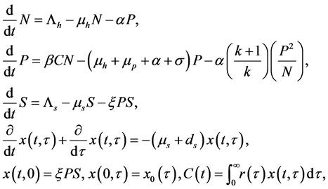
Therefore, we have the following four-dimensional limit system of system (3) which summarizes the above result.

(6)

The existence and the uniqueness of solutions of system (6) can be proved by using standard methods (see, for example, [24] ).

3. Equilibrium States

In this section, the equilibrium states of system (6) are discussed. The system (6) admits two steady states. We establish sufficient condition for the globally asymptotic stable of infection-free solution and for the permanence of the system (6).

3.1. Boundedness

The model (6) describes the dynamics of adult parasites and snail. It is important to prove that these populations are positive and bounded for with any positive initial data. So we have the following results.

Theorem 1. If is any solution of system (6), and, , and, then, , , for all.

Proof. From the first equation of system (6), we have

After integrating, we obtain

Similarly,

and

Hence, we conclude that the solution of system (6) is always positive for all.

Theorem 2. For any nonnegative initial data, the solution of system (6) are bounded for all time.

Proof. From the last two equations in system (6), we have

Consider the comparison system

It is easy to see that as. Thus

(7)

It follows from the first and second equations of (6) and (7) that

Similarily above, and is a ultimately upper bound of and, respectively. The proof is completed.

The equilibrium states of the basic model are obtained by setting the right-hand side of system (6) to zero. The system (6) has two steady states of the disease-free equilibrium and the endemic equilibrium.

3.2. The Disease-Free Equilibrium

At the disease-free state, there is no adult parasitrs and infected snails and hence no infection in the host and the intermediate host. Thus, the system (6) has a disease-free equilibrium

where

In many epidemic models, the basic reproductive number is a key parameter. It refers to the expected number of secondary infections during the entire period of infectiousness in a completely susceptible population [25] . Following the idea in [26] , we give the basic reproductive number for system (6). Rewrite system (6) as following form:

where. S denotes the number of uninfected snails, while components of Y represent the number of adult parasites that are hosted by human hosts in Village, and infected snails, respectively. Following the symbol in [26] , we compute matrixes A, M and D as

(8)

where. Obviously, and is a diagonal matrix. The basic reproductive number is the spectral radius (dominant eigenvalue) of the matrix, that is,

Thus, in this case

(9)

where

and

We know that presents the schistosomiasis transmission coefficient in village 1, and represents the schistosomiasis transmission coefficient in village 2.

From above discussion, we have following result.

Theorem 3. The disease-free equilibrium point is locally asymptotically stable if and unstable if.

Next, we give two conditions which guarantee the global asymptotic stability of the disease-free state.

(H1) For, is globally asymptotically stable.

(H2), for, where, is an M-matrix.

For system (6), we have

and A is given in (8). It is clear that for all. It is easy to see that the conditions (H1) and (H2) hold. According to the result of literature [26] , we have the following result.

Theorem 4. The disease-free equilibrium is globally asymptotically stable provided that and the assumptions (H1) and (H2) are satisfied.

3.3. The Endemic Equilibrium

First, we show the existence of the unique endemic equilibrium when. Ex- pressing in terms of, we can derive from system (6) as follows.

Substituting the expressions for, and into the fourth equation of system (6) we get

(10)

where

By solving (10) for we get one of the solutions as which corresponds to the disease-free equilibrium. For implies that. Since, then the endemic equilibrium exists. The results of the existence of the endemic equilibrium of system (6) can be summarized in the following lemma.

Lemma 5. The system (6) always has a disease-free equilibrium and a unique endemic equilibrium when.

Center Manifold Theory [19] has been used to determine the local stability of a nonhyperbolic equilibrium, we now employ the Center Manifold Theory to establish the local asymptotic stability of the endemic equili- brium. In order to apply the Center Manifold Theory, we make the following change of variables. Let, , ,. Now we use the vector notation. Then the system (6) is written in following form

such that

(11)

Evaluating the Jacobian matrix of system (11) at the disease-free equilibrium, it can be shown that the reproduction number is

Take as the bifurcation parameter. Considering the case and solving for, we get

We notice that the linearized system (11) of the transformed equation with, has a simple zero eigenvalue. Hence, Center Manifold Theory can be used to analyze the dynamics of (13) near. By Theorem 4.1 in Castillo-Chavez and Song [27] , it can be shown that the Jacobian matrix at has a right eigenvector of associated with the zero eigenvalue given by, where

The left eigenvector of associated with the zero eigenvalue at is given by, where

We now use the following lemma whose proof is found in [27] .

Lemma 6. Consider the following general system of ordinary differential equations with a parameter,

(12)

where 0 is an equilibrium of the system, that is for all and assume

A1: is the linearization of system (12) around the equilibrium 0 with

evaluated at 0. Zero is a simple eigenvalue of A and other eigenvalues of A have negative real parts;

A2: Matrix A has a right eigenvector u and a left eigenvector v corresponding to the zero eigenvalue. Let be the kth component of f and

(13)

The local dynamics of (12) around 0 are totally governed by a and b.

1). when with, 0 is locally asymptotically stable, and there exists a positive unstable equilibrium; when, 0 is unstable and there exists a negative and locally asymptotically stable equilibrium;

2). when with, 0 is unstable; when, 0 is locally asymptotically stable, and there exists a positive unstable equilibrium;

3). when with, 0 is unstable, and there exists a locally asymptotically stable negative equilibrium; when, 0 is stable and a positive unstable equilibrium appears;

4). When changes from negative to positive, 0 changes its stability from stable to unstable. Correspondingly a negative unstable equilibrium becomes positive and locally asymptotically stable.

We now compute a and b, for system (11), the associated non-zero partial derivatives of at the disease free equilibrium are given by

Substituting the above expressions into (13), we get

For the sign of b, it is associated with the following non-vanishing partial derivatives of,

It follows from the above expression that

Thus, and. According to Lemma 6, item (iv), we can yield the following result which only holds for, but close to 1.

Theorem 7. The unique endemic equilibrium is locally asymptotically stable for near 1.

In summary, model (6) has a disease-free equilibrium which is globally asymptotically stable when, and a unique endemic equilibrium point when. The unique endemic equilibrium is locally asymptotically stable at least near. We use numerical simulations to show the existence and stability of endemic equilibrium.

4. Numerical Simulations and Control Strategies

In this section, in order to understand our results more intuitively, some numerical simulations of system (6) that support and extend the conclusions of previous sections are carried out. We use year as unit of time, and choose the parameters, , , , , , , , , , , , , , ,.

In Figure 1, we show the relationship between the threshold and adult parasites for the mathematical model (6). It is easy to see that is a bifurcation point, and the adult parasites are stable eventually, when the threshold increases. Otherwise, the adult parasites are extinct. It implies that the threshold is greater than unit, the schistosomiasis will be endemic. Figure 1 and Figure 2 show that if the threshold is less than unit, the schistosomiasis will be extinct.

Figure 1. The relationship between the threshold and for system (6).

Figure 2. Time series of solutions for system (6). The disease will be extinct eventually..

To see the relative effect of migration in each village, we plot the curved surface of the relationship between, and. From Figure 3 and Figure 4, we can observe that decreases dramatically when increases and is fixed with a small number, and increases sharply when increases and is fixed with a small number. This implies that the migration from severe endemic village to mild endemic village is bad for disease control.

In Figure 5, we consider the infection rates, and as the control factors. We plot the curved surface of the threshold as a function of and. We observe that the threshold decreases dramatically when and decrease. It means that decreasing infection rates is helpful to prevent schistosomiasis transmission.

5. Conclusion and Discussion

As a kind of the tropical diseases, schistosomiasis continues to be a significant public health threat in the world.

Figure 3. It shows sensitive figure that the relationship between the threshold and migrated rate,.

Figure 4. The relationship between the threshold and migrated rate,.

Figure 5. It shows sensitive figure that the relationship between the threshold and migrated rate,.

Following the pioneering work of Feng et al. [16] on modeling schistosomiasis, we establish and analyzed a schistosomiasis model with diffusion effect and saturated incidence function, in which two groups of human share the water contaminated by schistosomiasis and migrate each other. we derived the basic reproduction number and proved that the disease-free equilibrium is globally asymptotically stable when, and the unique endemic equilibrium is locally asymptotically stable for is larger than 1 and near 1. Our results indicate that the diffusion rates and the infection rates play an important role in the determination of the permanence and extinction of schistosomiasis. The diffusion from the mild endemic village to severe endemic village is benefit to control schistosomiasis transmission.

In realistic situations, there might be several human groups sharing the contaminated water resource. Only considering the model with two human groups is insufficient, we expect a similar to work in higher-dimensional systems with n human groups and migration. It can be guessed that the model with n human groups has similar mathematical properties to two human groups.

Acknowledgements

The research has been supported by The Natural Science Foundation of China (11561004, 11261004), The Supporting the Development for Local Colleges and Universities Foundation of China-Applied Mathematics Innovative Team Building, the 12th Five-year Education Scientific Planning Project of Jiangxi Province (15ZD3LYB031), The Natural Science Foundation of Jiangxi Province (20151BAB201016) and the Social Science Planning Projects of Jiangxi Province (14XW08).

Conflicts of Interest

The authors declare no conflicts of interest.

References

[1]	Ross, A.G.P., Bartley, P.B., Sleigh A.C., et al. (2002) Schistosomiasis. The New England Journal of Medicine, 346, 1212-1220. http://dx.doi.org/10.1056/NEJMra012396
[2]	Croft, S.L., Vivas, L. and Brooker, S. (2003) Recent Advances in Research and Control of Malaria, Leishmaniasis, Trypanosomiasis and Schistosomiasis. Eastern Mediterranean Health Journal, 9, 518-533.
[3]	Huang, Y.-X. and Manderson, L. (2005) The Social and Economic Context and Determinants of Schistosomiasis Japonica. Acta Tropica, 96, 223-231. http://dx.doi.org/10.1016/j.actatropica.2005.07.015
[4]	Thétiot-Laurent, S.A.L., Boissier, J., Robert, A. and Meunier, B. (2013) Schistosomiasis Chemotherapy. Angewandte Chemie International Edition, 52, 7936-7956. http://dx.doi.org/10.1002/anie.201208390
[5]	Patz, J.A., Graczyk, T.K., Geller, N., et al. (2000) Effects of Environmental Change on Emerging Parasitic Diseases. International Journal for Parasitology, 30, 1395-1405. http://dx.doi.org/10.1016/S0020-7519(00)00141-7
[6]	Zhang, S.-M., Lv, Z.-Y., Zhou, H.-J., et al. (2008) Characterization of a Profilin-Like Protein from Schistosoma Japonicum, a Potential New Vaccine Candidate. Parasitology Research, 102, 1367-1374. http://dx.doi.org/10.1007/s00436-008-0919-2
[7]	McManus, D.P., Gray, D.J., Li, Y., et al. (2010) Schistosomiasis in the People’s Republic of China: The Era of the Three Gorges Dam. Clinical Microbiology Reviews, 23, 442-466. http://dx.doi.org/10.1128/CMR.00044-09
[8]	Ross, A.G., Sleigh, A.C., Li, Y., et al. (2001) Schistosomiasis in the People’s Republic of China: Prospects and Challenges for the 21st Century. Clinical Microbiology Reviews, 14, 270-295. http://dx.doi.org/10.1128/CMR.14.2.270-295.2001
[9]	Luo, R., Zhou, C., Lin, J., et al. (2012) Identification of in Vivo Protein Phosphorylation Sites in Human Pathogen Schistosoma Japonicum by a Phosphoproteomic Approach. Journal of Proteomics, 75, 868-877. http://dx.doi.org/10.1016/j.jprot.2011.10.003
[10]	The Schistosoma japonicum Genome Sequencing and Functional Analysis Consortium (2009) The Schistosoma Japonicum Genome Reveals Features of Host-Parasite Interplay. Nature, 460, 345-351. http://dx.doi.org/10.1038/nature08140
[11]	Macdonald, G. (1965) The Dynamics of Helminth Infections, with Special Reference to Schistosomes. Transactions of the Royal Society of Tropical Medicine & Hygiene, 59, 489-506. http://dx.doi.org/10.1016/0035-9203(65)90152-5
[12]	N?sell, I. and Hirsch, W.M. (1973) The Transmission Dynamics of Schistosomiasis. Communications on Pure and Applied Mathematics, 26, 395-453. http://dx.doi.org/10.1002/cpa.3160260402
[13]	Woolhouse, M.E. (1992) On the Application of Mathematical Models of Schistosome Transmission Dynamics 2. Control. Acta Tropica, 50, 189-204. http://dx.doi.org/10.1016/0001-706X(92)90076-A
[14]	Liang, S., Maszle, D. and Spear, R.C. (2002) A Quantitative Framework for a Multi-Group Model of Schistosomiasis Japonicum Transmission Dynamics and Control in Sichuan, China. Acta Tropica, 82, 263-277. http://dx.doi.org/10.1016/S0001-706X(02)00018-9
[15]	Feng, Z., Li, C.C. and Milner, F.A. (2005) Schistosomiasis Models with Two Migrating Human Groups. Mathematical and Computer Modelling, 41, 1213-1230. http://dx.doi.org/10.1016/j.mcm.2004.10.023
[16]	Feng, Z., Li, C.C. and Milner, F.A. (2002) Schistosomiasis Models with Density Dependence and Age of Infection in Snail Dynamics. Mathematical Biosciences, 177-178, 271-286. http://dx.doi.org/10.1016/S0025-5564(01)00115-8
[17]	Bhattacharyya, R. and Mukhopadhyay, B. (2010) Analysis of Periodic Solutions in an Eco-Epidemiological Model with Saturation Incidence and Latency Delay. Nonlinear Analysis: Hybrid Systems, 4, 176-188. http://dx.doi.org/10.1016/j.nahs.2009.09.007
[18]	Xu, R. and Du, Y. (2009) A Delayed Sir Epidemic Model with Saturation Incidence and a Constant Infectious Period. Journal of Applied Mathematics and Computing, 35, 229-250. http://dx.doi.org/10.1007/s12190-009-0353-3
[19]	Carr, J. (1981) Applications of Centre Manifold Theory. Applied Mathematical Sciences, 35, 1-36. http://dx.doi.org/10.1007/978-1-4612-5929-9
[20]	Yu, X., Wu, C. and Weng, P. (2012) Traveling Waves for a Sirs Model with Nonlocal Diffusion. International Journal of Biomathematics, 05, 1250036. http://dx.doi.org/10.1142/S1793524511001787
[21]	Liu, J., Zhou, H. and Zhang, L. (2012) Cross-Diffusion Induced Turing Patterns in a Sex-Structured Predator-Prey Model. International Journal of Biomathematics, 5, 1250016. http://dx.doi.org/10.1142/S179352451100157X
[22]	Chen, S., Shi, J. and Wei, J. (2012) Time Delay-Induced Instabilities and Hopf Bifurcations in General Reaction-Diffusion Systems. Journal of Nonlinear Science, 23, 1-38. http://dx.doi.org/10.1007/s00332-012-9138-1
[23]	Chiyaka, E.T. and Garira, W. (2009) Mathematical Analysis of the Transmission Dynamics of Schistosomiasis in the Human-Snail Hosts. Journal of Biological Systems, 17, 397-423. http://dx.doi.org/10.1142/S0218339009002910
[24]	Hale, J.K. (1969) Ordinary Differential Equations. Applied Mathematical Sciences, John Wiley & Sons Inc, New Jersey, 12-20.
[25]	Anderson, R.M. and May, R.M. (1991) Infectious Diseases of Humans: Dynamics and Control. Oxford University Press, Oxford.
[26]	Chavez, C.C., Feng, Z. and Huang, W. (2002) On the Computation of R0 and Its Role in Global Stability. In: Mathematical Approaches for Emerging and Re-Emerging Infection Diseases: An Introduction. The IMA Volumes in Mathematics and Its Applications, Vol. 125, Springer, New York, 31-65.
[27]	Castillo-Chavez, C. and Song, B. (2004) Dynamical Models of Tuberculosis and Their Applications. Mathematical Biosciences and Engineering: MBE, 1, 361-404. http://dx.doi.org/10.3934/mbe.2004.1.361