DEA Scores’ Confidence Intervals with Past-Present and Past-Present-Future Based Resampling ()
Received 8 January 2016; accepted 5 March 2016; published 8 March 2016

1. Introduction
DEA is a non-parametric methodology for performance evaluation and benchmarking. Since the publication of the seminal paper by Charnes, Cooper and Rhodes [1] , DEA has witnessed numerous developments, some of which are motivated by theoretical considerations and others motivated by practical considerations. The focus of this paper is on practical considerations related to data variations. The first practical issue is the lack of a statistical foundation for DEA which was laid down by Banker [2] who proved that DEA models could be viewed as maximum likelihood estimation models under specific conditions and then Banker and Natarajan [3] proved that DEA provides a consistent estimator of arbitrary monotone and concave production functions when the (one- sided) deviations from such a production function are degraded as stochastic variations in technical inefficiency. Afterwards the treatment of data variations has taken a variety of forms in DEA. In fact, several authors investigated the sensitivity of DEA scores to data variations in inputs and/or outputs using sensitivity analysis and super-efficiency analysis. For example, Charnes and Neralić [4] and Neralić [5] used conventional linear programming-based sensitivity analysis under additive and multiplicative changes in inputs and/or outputs to investigate the conditions under which the efficiency status of an efficient DMU is preserved (i.e., basis remains unchanged), whereas Zhu [6] performed sensitivity analysis using various super-efficiency DEA models in which a test DMU is not included in the reference set. This sensitivity analysis approach simultaneously considers input and output data perturbations in all DMUs, namely, the change of the test DMU and the remaining DMUs. On the other hand, several authors investigated the sensitivity of DEA scores to the estimated efficiency frontier. For example, Simar and Wilson [7] [8] used a bootstrapping method to approximate the sampling distributions of DEA scores and to compute confidence intervals (CIs) for such scores. Barnum et al. [9] provided an alternative methodology based on Panel Data Analysis (PDA) for computing CIs of DEA scores; in sum, they complemented Simar and Wilson’s bootstrapping by using panel data along with generalized least squares models to correct CIs for any violations of the standard statistical assumptions (i.e., DEA scores are independent and identically distributed, and normally distributed) such as the presence of contemporaneous correlation, serial correlation and heteroskedasticity. Note, however, that [7] and [8] do not take account of data variations in inputs and outputs. Note also that although [9] takes account of data variations in inputs and outputs by considering panel data and computing DEA scores separately for each cross section of the data, the reliability of the approach depends on the amount of data available for estimating the generalized least squares models.
In this paper, we follow the principles stated in Cook, Tone and Zhu [10] and believe that DEA performance measures are relative, not absolute, and frontiers-dependent. DEA scores undergo a change depending on the choice of inputs, outputs, DMUs and DEA models by which DMUs are evaluated. In this paper, we compute efficiency scores or equivalently solve the frontier problem using the non-oriented slacks-based super-efficiency model. Our approach deals with variations in both the estimated efficiency frontier and the input and output data directly by resampling from historical data over two different time frames (i.e., past-present and past-present- future); thus, the production possibility set for the entire DMUs differs with every sample1. In addition, our approach works for both small and large sets of data and does not make any parametric assumptions. Hence, our approach presents another alternative for computing confidence intervals of DEA scores.
This paper unfolds as follows. Section 2 presents a generic methodological framework to estimate the confidence intervals of DEA scores under a past-present time frame and extends it to the past-present-future time frame. Section 3 presents a healthcare application to illustrate the proposed resampling framework. Finally, section 5 concludes the paper.
2. Proposed Methodology
2.1. Past-Present Based Framework
The first framework is designed for when past-present information on say m inputs and s outputs of a set of n
DMUs is available; that is,  , where period T
denote the present and periods 1 though  represent the past. The proposed framework could be summarized as follows:
Initialization Step
Choose an appropriate DEA model for computing the efficiency scores of DMUs;
Use the chosen DEA model to estimate the DEA scores of DMUs based on the present information; that is, . Let
. Let  denote such scores-in the iterative step, we gauge the confidence interval of
 using replicas of historical data
 ;
;
Choose an appropriate scheme, say w, to weigh the available information on the past and the present;
Choose a confidence level ;
;
Choose the number of replicas or samples to draw from the past, say B, along with any properties they should satisfy before being considered appropriate to use for generating the sampling distributions of  and computing their confidence intervals;
Set an indicator variable, say , that reflects whether the B replicas satisfy the required properties or not to false.
Iterative Step
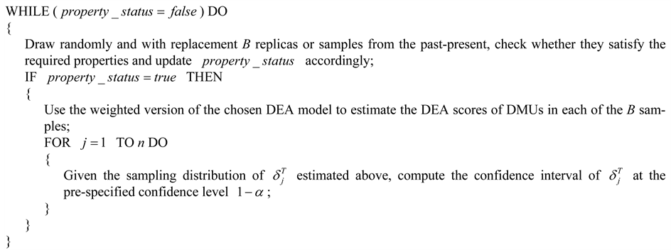
The generic nature of this framework requires a number of decisions to be made for its implementation for a particular application. Hereafter, we shall discuss how one might make such decisions.
2.1.1. Choice of a DEA Model
In principle one might choose from a relatively wide range of DEA models; however, given the nature of this exercise we recommend the use of the non-oriented super slacks-based measure model (Tone [12] and Ouenniche et al. [13] ) under the relevant returns-to-scale (RTS) setup (e.g., constant, variable, increasing, decreasing) as suggested by the RTS analysis of the dataset one is dealing with. This model is an extension of the SBM (slacks-based measure) model of Tone [14] ―see also [15] . Although one could use other models (e.g., radial or oriented), our recommendation is based on the following reasons. First, as a non-radial model, the SBM model is appropriate for taking account of input and output slacks which affect efficiency scores directly, whereas the radial models are mainly concerned with the proportional changes in inputs or outputs. Thus, SBM scores are more sensitive to data variations than the radial ones. Second, the non-oriented SBM model can deal with input-surpluses and output-shortfalls within the same scheme. Finally, as most DEA scores are bounded by unity (≤1, or ≥1), difficulties in comparing efficient DMUs maybe encountered; therefore, we recommend using the super-efficiency version of the non-oriented SBM as it removes such unity bounds.
2.1.2. Choice of a Weighting Scheme for Past-Present Information
2.1.3. Choice of the Replication Process and the Number of Replicas
In this paper, we regard historical data  as
as
discrete events with probability  and cumulative probability
 . We propose a repli-
cation process based on bootstrapping. First proposed by Efron [16] , nowadays bootstrapping refers to a collection of methods that randomly resample with replacement from the original sample. Thus, in bootstrapping, the population is to the sample what the sample is to the bootstrapped sample. Bootstrapping could be either parametric or non-parametric. Parametric bootstrapping is concerned with fitting a parametric model, which in our case would be a theoretical distribution, to the data and sampling from such fitted distribution. This is a viable approach for large datasets where the distribution of each input and each output could be reasonably approximated by a specific theoretical distribution. However, when no theoretical distribution could serve as a good approximation to the empirical one or when the dataset is small, non-parametric bootstrapping is the way to proceed. Non-parametric bootstrapping does not make any assumptions except that the sample distribution is a good approximation to the population distribution, or equivalently the sample is representative of the population. Consequently, datasets with different features require different resampling methods that take account of such features and thus generate representative replicas.
For a non-correlated and homoskedastic dataset, one could for example use smooth bootstrapping or Bayesian bootstrapping, where smooth bootstrapping generates replicas by adding small amounts of zero-centered random noise (usually normally distributed) to resampled observations, whereas Bayesian bootstrapping generates replicas by reweighting the initial data set according to a randomly generated weighting scheme. In this paper, we recommend the use of a variant of Bayesian bootstrapping whereby the weighting scheme consists of the Lucas number series-based weights  presented above, because it is more appropriate when one is resampling over a past-present time frame and more recent information is considered more valuable. For a non-correlated and homoskedastic dataset, our Data Generation Process (DGP) may be summarized as follows. First, a random number
  is drawn from the uniform distribution over the interval [0,1], then whichever cross section data
 ![]() so that
so that ![]() is resampled, where
is resampled, where![]() . This process is repeated as many times as necessary to produce the required number of valid replicas or samples.
. This process is repeated as many times as necessary to produce the required number of valid replicas or samples.
On the other hand, for a correlated and/or heteroskedastic dataset, one could use one of the block bootstrapping methods, where replicas are generated by splitting the dataset into non-overlapping blocks (simple block bootstrap) or into overlapping blocks of the same or different lengths (moving block bootstrap), sampling such blocks with replacement and then aligning them in the order they were drawn. The main idea of all block bootstrap procedures consists of dividing the data into blocks of consecutive observations of length![]() , say
, say
![]() , and sampling the blocks randomly with replacement from all possible
, and sampling the blocks randomly with replacement from all possible
Blocks―for an overview of bootstrapping methods, the reader is referred to [17] . The block bootstrap procedure with blocks of non-random length can be summarized as follows:
Input: Block length ![]() so that
so that![]() .
.
Step 1: Draw randomly and independently block labels, say![]() , from the set of labels, say L, where
, from the set of labels, say L, where![]() ,
, ![]() if non-overlapping blocks are considered, and
if non-overlapping blocks are considered, and ![]() if overlapping blocks are considered.
if overlapping blocks are considered.
Step 2: Lay the blocks![]() , end-to-end in the or-
, end-to-end in the or-
der sampled together and discard the last ![]() observations to form a bootstrap series
observations to form a bootstrap series ![]() .
.
Output: Bootstrap sample![]() .
.
As to the choice of the number of replicas B, there is no universal rule except that the larger the value of B the more stable the results. However, one should take into consideration the computational requirements; therefore, in practice, one would keep increasing the value of B until the simulation converges; that is, the results from a run do not change when adding more iterations.
2.1.4. Choice of the Properties the Replicas Should Satisfy
2.2. Past-Present-Future Time Based Framework
In the previous subsection, we utilized historical data ![]() to gauge the confidence interval of the last period’s scores. In this section, we forecast the “future”; namely,
to gauge the confidence interval of the last period’s scores. In this section, we forecast the “future”; namely, ![]() by using “past-present” data
by using “past-present” data ![]() and forecast the efficiency scores of the future DMUs along with their confidence intervals. In order to avoid repetition, hereafter we shall discuss how the past-present time based framework could be extended to the past-present-future context. First, we have to forecast the future; to be more specific, given the observed historical data
and forecast the efficiency scores of the future DMUs along with their confidence intervals. In order to avoid repetition, hereafter we shall discuss how the past-present time based framework could be extended to the past-present-future context. First, we have to forecast the future; to be more specific, given the observed historical data ![]() for a certain input
for a certain input ![]() and output
and output ![]() of a DMU
of a DMU![]() , we wish to forecast
, we wish to forecast![]() . There are several forecasting engines available for this purpose. Once these forecasts are obtained, we then estimate the super-efficiency score of the “future” DMU
. There are several forecasting engines available for this purpose. Once these forecasts are obtained, we then estimate the super-efficiency score of the “future” DMU ![]() using the non-oriented super slacks-based measure model. Finally, given the past-present- future inter-temporal data set
using the non-oriented super slacks-based measure model. Finally, given the past-present- future inter-temporal data set![]() , we apply the resampling scheme proposed in the previous section and obtain confidence intervals.
, we apply the resampling scheme proposed in the previous section and obtain confidence intervals.
3. An Application in Healthcare
In this study we utilize a dataset concerning nineteen Japanese municipal hospitals from 2007 to 2009 to illustrate how the proposed framework works. There are approximately 1000 municipal hospitals in Japan and there is large heterogeneity amongst them. We selected nineteen municipal hospitals with more than 400 beds. Therefore, this sample may represent larger acute-care hospitals with homogeneous functions. The data were collected from the Annual Databook of Local Public Enterprises published by the Ministry of Internal Affairs and Communications. For illustration purposes, we chose for this study two inputs; namely, Doctor ((I)Doc) and Nurse ((I)Nur), and two outputs; namely, Inpatient ((O)In) and Outpatient ((O)Out). Table 1 exhibits the data, while Table 2 shows the main statistics. The data are the yearly averages of the fiscal year data, as we have no daily or monthly data, and the Japanese government’s fiscal year begins on April 1 and ends on March 31. As can be seen, the data on inputs and outputs fluctuate by year, which suggests the need for analysis of data variation.
We solved the non-oriented super slacks-based measure model year by year and obtained the super-efficiency scores in Table 3 along with their graphical representation in Figure 1. As can be seen, the scores fluctuate by year. Once again, this suggests the need for analysis of data variation. If we had daily data, this could be done. However, we only have fiscal-year data and hence we need to resample data in order to gauge the confidence interval of efficiency scores. Then, we merged the dataset of all years and evaluated the efficiency scores relative to 57 (![]() ) DMUs as exhibited in Table 4 and Figure 2. Comparing the averages of these three years, we found that the average 0.820 of year 2007 is better than 2008 (0.763) and 2009 (0.732). We also performed the non-parametric Wilcoxon rank-sum test and the results indicate that the null hypothesis; that is, 2007 and 2008 have the same distribution of efficiency scores, is rejected at the significance level 1%; therefore, 2007 outperforms 2008. Similarly, 2007 outperforms 2009. However, we cannot see significant difference between 2008 and 2009.
) DMUs as exhibited in Table 4 and Figure 2. Comparing the averages of these three years, we found that the average 0.820 of year 2007 is better than 2008 (0.763) and 2009 (0.732). We also performed the non-parametric Wilcoxon rank-sum test and the results indicate that the null hypothesis; that is, 2007 and 2008 have the same distribution of efficiency scores, is rejected at the significance level 1%; therefore, 2007 outperforms 2008. Similarly, 2007 outperforms 2009. However, we cannot see significant difference between 2008 and 2009.
3.1. Illustration of the Past-Present Framework
We applied the proposed procedure to the historical data of nineteen hospitals for the two years 2008-2009 in Table 1. We excluded the year 2007 data, because they belong to a different population than 2009 as explained in Preliminary results (Panel). Note that historical data may suffer from accidental or exceptional events, for example, oil shock, earthquake, financial crisis, environmental system change and so forth. We must exclude these from the data. If some data are under age depreciation, we must adjust them properly. In this study, we use Lucas weights for past and present data. However, we can use other weighting schema (e.g., exponential) as well.
Table 5 shows the correlation matrix of the observed 2009 year data in Table 1 and Fisher 95% confidence intervals are exhibited in Table 6. For example, the correlation coefficient between Doc and Outpatient is
![]()
Table 3. Super-SBM scores by cross section (year).
![]()
Table 4. Super-SBM scores for panel data (all years).
![]()
Table 6. Fisher 95% confidence lower/upper bounds for correlation matrix.
![]()
Figure 1. Super-SBM scores by cross section (year).
![]()
Figure 2. Super-SBM Scores for panel data (all years).
0.5178 and its 95% lower/upper bounds are respectively 0.0832 and 0.7869. In addition, we report Fisher 20% confidence lower/upper bounds in Table 7. The intervals are considerably narrowed down compared with Fisher 95% case.
Table 8 exhibits results obtained by 500 replicas where the column DEA is the last period’s (2009) efficiency score and Average indicates the average score over 500 replicas. The column Rank is the ranking of average scores. We applied Fisher 95% threshold and found no out-of-range samples. Figure 3 shows the 95% confidence intervals for the last period’s (2009) DEA scores along with Average scores. The average of the 95% confidence interval for all hospitals is 0.10.
In the Fisher 95% (ζ95) case, we found no discarded samples, whereas in the Fisher 20% (ζ20) case, 1945 samples were discarded before getting 500 replicas. Table 9 shows the comparisons of scores calculated by both thresholds, where we cannot see significant differences.
Note that one resample produces one efficiency score for each DMU. We compared 500 and 5000 replicas and obtained the 95% confidence interval as exhibited in Table 10. As can be seen, the difference is negligibly small. 500 replicas may be acceptable in this case. However, the number of replicas depends on the numbers of
![]()
Table 7. Fisher 20% confidence lower/upper bounds for correlation matrix.
![]()
Table 8. DEA score and confidence interval with 500 replicas.
![]()
Table 9. Comparisons of Fisher’s 20% (ζ20) and 95% (ζ95) thresholds.
![]()
Table 10. Comparisons of 5000 and 500 replicas (Fisher 95%).
inputs, outputs and DMUs. Hence, we need to check the variations of scores by increasing the number of replicas.
Finally, we would like to draw the reader’s attention to the fact that, in some applications, one might set weights to inputs and outputs. Actually, if costs for inputs and incomes from outputs are available, we can evaluate the comparative cost performance of DMUs. In the absence of such information, instead, we can set weights to inputs and outputs. For example, the weights to Doc and Nurse are assumed to be 5 to 1 (on average), and those of Outpatient to Inpatient are 1 to 10 (on average). We can solve this problem via the Weighted-SBM model, which will enhance the reliability and applicability of our approach.
3.2. Illustration of the Past-Present-Future Framework
Hereafter, we shall present numerical results for the past-resent-future framework. In this case we regard 2007- 2008 as the past-present and 2009 as the future. In our application, we used three simple prediction models to forecast the future; namely, a linear trend analysis model, a weighted average model with Lucas weights, and a hybrid model that consists of averaging their predictions.
Table 11 reports the forecasts for 2009 obtained by the linear trend analysis model. Table 12 shows the forecast DEA score and confidence interval along with the actual super-SBM score for 2009. Figure 4 exhibits 97.5% percent, 2.5% percent, forecast score and actual score. It is observed that, of the nineteen hospitals, the actual 2009 scores of sixteen are included in the 95% confidence interval. The average of Forecast-Actual over the nineteen hospitals was 0.063 (6.3%).
Table 13 reports 2009 forecasts by the weighted average model with Lucas weights and Table 14 shows the actuals and the forecasts of 2009 scores along with confidence intervals. In this case, only four hospitals are included in the 95% confidence interval. The average of Forecast-Actual over the nineteen hospitals was 0.056 (5.6%). Although we did not report the results by the Average of Trend and Lucas case, the results are similar to the Lucas case. We compare the number of fails for the three forecast models that actual score is out of 97.5% and 2.5% interval. We have results as exhibited in Table 15. “Trend” gives the best performance among the three in this example.
4. Conclusion
DEA, originated by Charnes and Cooper (Charnes et al. [1] ), is a non-parametric mathematical programming methodology that deals directly with input/output data. Using the data, DEA can evaluate the relative efficiency
![]()
Table 11. 2009 forecasts: linear trend model.
![]()
Table 12. Forecast DEA score, actual (2009) score and confidence interval: forecast by linear trend model.
![]()
Table 13. 2009 forecasts: Lucas weighted average model.
![]()
Table 14. DEA score and confidence interval forecasts: Lucas weighted average model.
![]()
Figure 4. Confidence interval, forecast score and actual 2009 score: forecast by linear trend model.
of DMUs and propose a plan to improve the inputs/outputs of inefficient DMUs. This function is difficult to achieve with similar models in statistics, e.g., stochastic frontier analysis. DEA scores are not absolute but relative. They depend on the choice of inputs, outputs and DMUs as well as on the choice of model for assessing DMUs. DEA scores are subject to change and thus data variations in DEA should be taken into account. This subject should be discussed from the perspective of the itemized input/output variations. From this point of view, we have proposed two models. The first model utilizes historical data for the data generation process, and hence this model resamples data from a discrete distribution. It is expected that, if the historical data are volatile widely, confidence intervals will prove to be very wide, even when the Lucas weights are decreasing depending on the past-present periods. In such cases, application of the moving-average method is recommended. Rolling simulations will be useful for deciding on the choice of the length of the historical span. However, too many past year data are not recommended, because environments, such as healthcare service systems, are changing rapidly. The second model aims to forecast the future efficiency and its confidence interval. For forecasting, we used three models; namely, the linear trend model, the weighted average, and their average. On this subject, Xu and Ouenniche [19] [20] will be useful for the selection of forecasting models, and Chang et al. [21] will provide useful information on the estimation of the pessimistic and optimistic probabilities of the forecast of future input/output values.
NOTES
![]()