A Note on Differential Equation with a Large Parameter

S. O. Maliki, R. N. Okereke

Department of Mathematics Michael Okpara, University of Agriculture, Umudike, Nigeria.

DOI: 10.4236/am.2016.73018                

Abstract

We present here asymptotic solutions of equations of the type , where is a large parameter. The Bessel differential equation is considered as a typical example of the above and the solutions are provided as . Furthermore, the behaviour of the solutions as well as the stability of the Bessel ode is investigated numerically as the parameter grows indefinitely.

Keywords

ODE, Asymptotic Solutions, Bessel Differential Equation, Stability, MathCAD Solution

Received 23 October 2015; accepted 22 February 2016; published 25 February 2016

1. Introduction

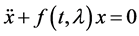
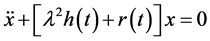
The theory of ordinary homogeneous linear differential equations of the second order, containing a large parameter, is well established [1] - [4] . The aim of this paper is to investigate detailed analytical solutions of equations of the form;

(1.1)

where is and is a real parameter. We shall investigate the behaviour of solutions of this differential equation, and the stability of the origin as. Without loss of generality, we take First, we make the following remarks:

a) Any second order linear ODE of the form; 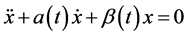can be reduced to by a suitable transformation.

b) Furthermore, any equation of the form is conservative. We shall demonstrate this shortly. This will help us in our asymptotic stability analysis.

c) In Equation (1.1) if we take; then, we have the well known Sturm-Liouville problem;

(1.2)

where, is positive and of class and.

Introducing the new variables;

(1.3)

If we suppress the variable t for the moment, it then follows that;

Therefore

Since, then, and after transforming the interval into, with further algebraic manipulations, the ode (1.2) becomes;

(1.4)

where

(1.5)

is a continuous function of. It can be shown that the solutions of (1.3) satisfy the Volterra integral equation;

(1.6)

where and are arbitrary. and have the same value, and the same derivate, at. The solution to the integral Equation (1.5) can be obtained by successive approximation in the form;

(1.7)

where;

Assuming that the function is bounded, i.e., there exists a constant M such that, then, one can show by induction that;

In the case of a finite interval, it follows that (1.7) is uniformly convergent for, and is also an asymptotic expansion of as. Unfortunately, the is very difficult to compute. Other approximations for large may be obtained from formal solutions, and these are usually divergent.

2. Formal Solutions

Let us now consider the general ode;

(2.1)

If is a formal power series in with coefficients which depend on x, then two linearly independent solutions of (2.1) may also be represented by a formal power series in. However if the formal expansion of in powers of contains positive powers of, then the formal expansion of x will be a Laurent series. We shall discover that in the case that, as a function of, has a pole at, we can still construct formal solutions.

In (2.1), we shall assume that is of the form;

(2.2)

where the are independent of, and Furthermore, we assume that does not vanish in the interval over which t varies. We shall adopt a first formal solution of the form;

(2.3)

Substituting (2.3) into (2.1), with the convention that for and for and also for All summations may then be assumed over all the integers, and we obtain

Picking out the coefficients of we obtain;

(2.4)

.

This first condition arises when Setting in (2.4) we obtain;

It then follows that;

(2.5)

(2.6)

.

Consequent upon these relations, we may restrict our summation to in the first sum in Equation (2.4). Now for in (2.4) we get;

(2.7)

and when we replace n by in (2.4) we obtain

(2.8)

It is now obvious that Equation (2.3) satisfies (2.1), provided that and satisfy (2.5) to (2.8).

In these equations, empty sums (i.e. those with upper limit

we may choose a branch of, and then (2.5) determines up to an additive constant. Moreover,

, and hence (2.6) determines recurrently, up to an additive constant in each. Equation (2.7) determines up to a constant factor, and (2.8) determines recurrently, up to an additive con-

stant multiple of in each. Corresponding to the two branches of, we obtain two formal solutions of the form (2.3).

3. Another Formal Solution

A second type of formal solution is given by

(2.9)

Substituting (2.9) into (2.1) we get;

Equating coefficients of,

(2.10)

(2.11)

(2.12)

There are two linearly independent formal solutions of this type. The obvious connection between these two types of formal solutions can be seen from the fact that equations (2.10) and (2.11) are identical with (2.5) and

(2.6), and is the formal expansion of.

3.1. Remark

In the foregoing, we have assumed that as a function of, has a pole of even order at. If the pole is of odd order, then no solution of the form (2.3) or (2.9) exists, and instead of powers of, we must expand in powers of.

3.2. Asymptotic Solutions

We shall now demonstrate that under certain assumptions, the differential Equation (2.1) possesses a fundamental system of solutions which are represented asymptotically by the formal solutions obtained in preceding section. It actually does not matter whether we compare solution of (2.1) with

where the and satisfy (2.5) to (2.8), or with

where the satisfy (2.10) to (2.12), for the q’s and’s can be so chosen that the ratio of these two expressions is.

We now fix a positive integer N, and set;

(3.1)

with, and for each j, the satisfy (2.10) to (2.12). These coefficients are completely determined by, and certain derivatives of these functions, and we shall say that the are sufficiently often differentiable if all the derivatives entering the determination of the exist and are continuous functions of t. We allow t to vary over a bounded and closed interval, and over a sectorial domain. We have the following theorem.

3.3. Theorem

Let S and I be as defined above then for each fixed is a continuous function of t over I; If

(3.2)

Uniformly in t and, as in S, where the are sufficiently often differentiable in I, and

(3.3)

, then the differential equation

(3.4)

possesses a fundamental system of solutions, and, such that

,

(3.5)

Proof

Top establish the existence and asymptotic property of, we substitute

(3.6)

in Equation (3.4) to get

(3.7)

where

(3.8)

uniformly in t and in S, by (3.2) and (2.10) to (2.12). Equation (3.7) may be written as

By two successive integrations, and a suitable choice of the constants of integration, we obtain;

(3.9)

where

Since is an increasing function, we have and .

The existence of follows immediately from the theory of Volterra integral equations, or can be established by successive approximations. From (3.8) and (3.9), we have, uniformly in t and in S. Furthermore is differentiable, i.e.

and

This proves (3.5) for. The proof for is very much similar, except that b rather than a, must be chosen as fixed limit of integration in the integral equation.

4. Application

The methods of the last two sections can be applied to prove the asymptotic formulae for the Bessel functions [1] , viz;

1)

2)

3)

Equation (1) holds for, uniformly in if

Equations (2) and (3) hold for uniformly in if

We observe that the functions; are solutions of the differential equation

(3.10)

This equation is of the form (3.4) with all other vanishing identically. The points are singular points of (3.10) and is a so called transition point at which the condition (3.3) is violated for any value.

5. Stability Analysis

In Section 1.0, we claimed that any equation of the form is conservative. It turns out that such systems are characterized by closed curves in the phase plane. For the former equation, we only need to show that it possesses a Hamiltonian H, such that.

Let us begin by multiplying the equation by, i.e.,

(3.11)

Observing that

Hence (3.11) becomes

Thus, the required Hamiltonian is.

The Bessel differential equation

can be recast in vector form as

Clearly the origin (0, 0) is the only critical point and the corresponding Hamiltonian is;

We use the above Hamiltonian to construct a Lyapunov function given by;

with and. We note that, furthermore;

Thus. Since, it follows that and hence the origin is asymptotically stable for all and.

6. Numerical Investigation of Asymptotic Solutions

In what follows, we employ the Runge-Kutta algorithm provided by MathCAD [5] software to obtain a numerical solution for large values of.

6.1. MathCAD Runge-Kutta Algorithm

We define the following for the MathCAD algorithm.

t₀: = 0.2 t₁: = 10 Solution interval endpoint

Initial condition vector

N: = 1500 Number of solution values on [t₀, t₁]

Derivative function

S: = rkfixed (ic, t₀, t₁, N, D) Runge-Kutta algorithm.

T: = S^<0> Independent variable values.

X₀: = S^<1> First solution function values.

X₁: = S^<2> Second solution function values.

Remark: X₀ represents solution values x satisfying the Bessel ODE, while X₁ represents the derivative of X₀ i.e.. S represents the j^th column vector in the solution matrix S, j = 0, 1, 2 (Figure 1).

6.2. Simulations

Figure 1. Section of solution matrix S.

6.3. Observations

For solutions no longer exist as they become unbounded. From the graphs shown, it is clear that the given Bessel differential equation is very sensitive to the parameter, and as the effect is to increase the oscillations until the solutions become unstable and die out. Furthermore, the phase portrait depicted shows that the Bessel differential equation represents a conservative system. This is clearly evident from the closed curves. However for, the phase portrait no longer appears like a closed curve but more like an explosion from the centre.

6.4. Conclusion

In this work, we have studied asymptotic solutions of equations of the type, where is a large parameter. We have shown that equations of this form represent a conservative system, meaning that they possess a conserved quantity, namely the Hamiltonian which is computed. As a special example, we consider the

Bessel differential equation for which the behaviour of the solutions as well as

the stability of the origin is investigated numerically as the parameter grows indefinitely.

Conflicts of Interest

The authors declare no conflicts of interest.

References

[1]	Olver, F.W.J. (1997) Asymptotics and Special Functions. Academic Press, New York. Reprinted by AK Peters, Wellesley.
[2]	Shkil, M.I. (1971) Asymptotic Methods in Differential Equations. Vyshcha Shkola, Kyiv, 228 p.
[3]	Territin, Kh.L. (1957) Asymptotic Expansion of Solutions to System of Ordinary Differential Equations Containing Parameter. Matematika: Sb. per., 1, 29-59.
[4]	Tikhonov, A. (1948) On Dependence of Solutions of Differential Equations on Small Parameter. Mat. Sb., 28, 193-204.
[5]	MathSoft, Inc. (1997) MathCAD 7 User’s Guide. http://www.mathsoft.com