Parametrization to Improve the Solution Accuracy of Problems Involving the Bi-Dimensional Dirac Delta in the Forcing Function ()
1. Introduction
One purpose of this paper is to emphasize the fact that the parametric delta is an exact representation, i.e., its value is zero everywhere except at one single point, and at that point its value is infinity. Another purpose is to illustrate the use and the effect of the parametric delta relating to two-dimensional domains, in space-time or in space-space; in these two cases, a product of deltas is involved, of course. Still another purpose is to present a problem example in which the operator action of the parametric delta facilitates the solution.
According to distribution theory, the Dirac delta is the result of differentiating the Heaviside unit step. The particular parametrization presented in [1] permits this differentiation to be carried out by means of elementary calculus and the resulting pair of parametric equations is exact and closed.
It is well to keep in mind that the parametric equations of the delta confirm that its area has unit value, that they comply with the fundamental property and that they yield the correct Laplace [1] and Fourier transforms [2] .
In the solution of differential equations, the parametric equations are handled exclusively by calculus and algebra, both at an elementary level. The parametrized representation can be readily visualized geometrically. These two features should make these parametric equations particularly convenient as a useful research tool, and also, for the purpose of teaching the Dirac delta concept at an early stage in undergraduate school.
1.1. Parametric Representation of the Dirac Delta
The parametric equations of the Dirac delta were developed by differentiating the unit step with a riser. The parametric representation of the unit step with a riser is given by [1] :
 (1)
(1)
 (2)
(2)
These two functions would be continuous were it not for the fact that they are undetermined at the points  and
and , however, since their left limit is the same as their right limit at those points, they will be treated as if they were continuous because this “…is generally inconsequential in applications” [3] -[6] and ([5] , p. 114).
Where:
 (3)
(3)
is the Cauchy limiting coefficient [6] , equivalent to a unit step with derivative equal to zero
 (4)
(4)
It is clear then that differentiating  does not yield the Dirac delta. Thus, it follows that
 (5)
(5)
 (6)
(6)
Consequently:
 (7)
(7)
This is the parametric Dirac delta, a more rigorous derivation of which was presented in [2] where it was clearly established that its value is 0 for  and
and  and its value is infinity at the single point:
 .
.
1.2. Product of Two Parametric Deltas
Figure 1 is a parametric plot of 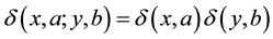 vs.
vs.  and
and . Since in
 ![]() in the range
in the range ![]() and
and ![]() in the range
in the range ![]() the value of the deltas is infinity; in order to avoid problems, instead of the value 1 in Equation (7) a value of 1.00000001 was used for plotting purposes. It was possible to obtain this plot because fortunately Mathematica 4.1 leaves a trace.
the value of the deltas is infinity; in order to avoid problems, instead of the value 1 in Equation (7) a value of 1.00000001 was used for plotting purposes. It was possible to obtain this plot because fortunately Mathematica 4.1 leaves a trace.
2. Examples
2.1. Example 1
Determine the deflection of a thin rectangular membrane clamped on all four edges and loaded by a force applied at point![]() .
.
“Solution:” The deflection is governed by the Poisson equation:
![]() (8)
(8)
Subject to the boundary conditions:
![]() (9)
(9)
Nomenclature:
![]() deflection;
deflection;
x = position along the ![]() dimension of the membrane;
dimension of the membrane;
y = position along the ![]() dimension of the membrane;
dimension of the membrane;
a = location of the load in the x direction;
b = location of the load in the y direction;
u = x parameter;
v = y parameter;
P = load;
T = tension per unit length.
This problem will be solved by, what we will call, the Parametrized Eigenfunction Expansion Method.
Assuming that [7] :
![]() (10)
(10)
Substituting Equation (10) into Equation (8)
![]() (11)
(11)
where
![]() (12)
(12)
Equation (11) can be interpreted as the Fourier expansion of the product:![]() .
.
The Fourier coefficients are:
![]() (13)
(13)
or equivalently:
![]() (14)
(14)
introducing the parameters u and v:
![]() (15)
(15)
simplifying Equation (15):
![]() (16)
(16)
Substituting Equation (5) into Equation (16) results in
![]() (17)
(17)
with![]() ;
;![]() .
.
Or equivalently
![]() (18)
(18)
![]() (19)
(19)
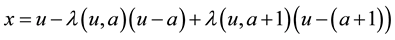
Therefore the parametric solution is:
![]() (20a)
(20a)
![]() (20b)
(20b)
![]() (20c)
(20c)
The non-parametric solution is Equation (20c), of course, notice that it is the same as the bilinear formula for Green’s function ([5] , pp. 520, 521). Figure 2 shows plots of the two solutions. Notice that the plot of the parametric solution clearly shows that the force is applied at a single point and that this is not the case in the plot of the non-parametric solution.
![]()
Figure 2. Plots of the solutions of the deflection of a clamped (on all four sides) membrane subject to a point force. (a) Parametric solution from Equations (20a), (20b) and (20c). (b) Non-parametric solution from the single Equation (20c). Both plots were obtained with 60 plot points.
2.2. Example 2
Consider a one dimensional rod subject to an impulsive heat source concentrated at point![]() ; with initial temperature of 0˚C along the full length of the rod and with the ends kept at 0˚C throughout the whole process. The specialized heat Equation ([8] , p. 381) is:
; with initial temperature of 0˚C along the full length of the rod and with the ends kept at 0˚C throughout the whole process. The specialized heat Equation ([8] , p. 381) is:
![]() (21)
(21)
Subject to the boundary conditions:
![]() (22)
(22)
![]() (23)
(23)
and to the initial condition
![]() (24)
(24)
Nomenclature:
T = temperature;
x = position along the rod;
t = time;
a = location of the heat source in the x direction;
u = position along the rod parameter;
w = time parameter;
Q = heat per unit area;
c = specific heat;
k = thermal conductivity;
ρ = mass density.
Solution: This problem will be solved by, what we will call, the Direct Parametric Method.
Separating the variables:
![]() (25)
(25)
Recalling that ![]() and substituting Equation (25) into Equation (21) yields
and substituting Equation (25) into Equation (21) yields
![]() (26)
(26)
Introducing the parameter w into Equation (26), yields:
![]() (27)
(27)
multiplying both sides of Equation (27) by![]() :
:
![]() (28)
(28)
Specializing Equations (5) and (6) yields:
![]() (29)
(29)
![]() (30)
(30)
Substituting Equations (29) and (30) into Equation (28), yields the control equation:
![]() (31)
(31)
or in accordance with Equation (25),
![]() (32)
(32)
During the impulse instant,![]() :
:
Equation (31) becomes
![]() (33)
(33)
Notice that, due to the parametric representation, the term referring to the energy conduction process has been eliminated by the operator action of the parametric delta, ![]() , Equations (29), (30) and (32). This is perfectly reconciled with physical reality, since during the impulse instant there is no time for conduction to take place. Furthermore, because of the operator action, the delta
, Equations (29), (30) and (32). This is perfectly reconciled with physical reality, since during the impulse instant there is no time for conduction to take place. Furthermore, because of the operator action, the delta ![]() itself has been replaced by 1.
itself has been replaced by 1.
According to the separation of variables method, Equation (33) implies
![]() (34)
(34)
where ![]() is a separation constant, thus:
is a separation constant, thus:
![]() (35)
(35)
and
![]() (36)
(36)
Integrating Equation (35) yields:
![]() (37)
(37)
substituting Equations (36) and (37) into Equation (25), yields
![]() (38)
(38)
At the “beginning” of the impulse instant, ![]() , and from the initial condition, Equation (24),
, and from the initial condition, Equation (24), ![]() , consequently Equation (38) becomes
, consequently Equation (38) becomes
![]() (39)
(39)
But ![]() [9] , thus
[9] , thus![]() . Then, Equation (38) becomes
. Then, Equation (38) becomes
![]() (40)
(40)
At the “end” of the impulse instant, w = 1, Equation (40) reduces to:
![]() (41)
(41)
At post impulse time,![]() :
:
The control Equation (32) becomes
![]() (42)
(42)
Notice that, due to the parametric representation, the post impulse equation is homogeneous because the forcing function has been eliminated by the operator action of the parametric delta, ![]() , Equations (29), (30) and (32).
, Equations (29), (30) and (32).
Which has the solution ([8] , p. 383).
:
![]() (43)
(43)
Because of continuity requirements, the temperature at the “beginning” of the post-impulse time must be equal to the temperature at the end of impulse instant.
![]() (44)
(44)
Thus the initial condition of post impulse time according to Equation (41) is
![]() (45)
(45)
Substituting Equations (41) and (43) into Equation (44), yields
![]() (46)
(46)
The right member of Equation (46) is recognized as the Fourier sine series of the left member; with coefficients
![]() (47)
(47)
Substituting Equation (7) into Equation (47),
![]() (48)
(48)
Substituting Equations (2), (5) and (6) into Equation (48),
![]() (49)
(49)
or equivalently,
![]() (50)
(50)
![]() (51)
(51)
Complete parametric solution:
Collecting Equations (40), (43) and (51), the parametric solution for ![]() may be expressed in the following form:
may be expressed in the following form:
![]() (52)
(52)
![]() (53)
(53)
Figure 3 is a plot of the solutions. Notice that the parametric solution represents correctly the initial condition of zero temperature and a vertical rise in temperature, as expected from an impulsive application of the heat source. In contrast, the non-parametric eigenfunction expansion solutions do not represent correctly the initial condition and, furthermore, the solution with 100 terms of the series, surprisingly, has a much greater error than that with only 20 terms of the series. Figure 4 is a plot of the parametric solution with a greater range of positive values of temperature than that of Figure 3(c), to show the effect of the product of the space and the time Dirac deltas.
![]()
Figure 3. (a) and (b) are plots of the solutions by the non-parametric eigenfunction expansion method, Equations (43) and (51): (a) with 20 terms of the series, (b) with 100 terms of the series. (c) Parametric solution with 100 terms of the series, Equations (52) and (53). 200 plot points were used in all three plots.
![]()
Figure 4. Plot of the parametric solution including a greater range of positive values of the temperature than in Figure 3(c), Equations (52) and (53) with 100 terms of the series and 200 plot points.
3. Further Comments Regarding the Solutions
The parametric Dirac delta representation was used to solve problems with forcing functions containing the product of two such deltas. The parametrized eigenfunction expansion method was used to solve problem (1) referring to the elastic deformation of a membrane subjected to a point load. The direct parametric method was used to solve problem (2) referring to the heat conduction in a metal rod subjected to the impulsive application of a concentrated heat source.
In the non-parametric eigenfunction expansion method, the integrals that constitute the values of the Fourier series coefficients contain the Dirac deltas. In the parametrized version, these deltas are substituted by the corresponding derivatives of the unit step and these, in turn, are expressed in terms of the parameters.
In the direct parametric method, in problems involving an impulsive forcing function represented by the time Dirac delta, the original differential equation is converted into two differential equations. The first of these equations refers to the impulse instant. Due to the operator action of the Dirac delta, the impulse instant equation may contain one term less than the original equation; furthermore, the Dirac delta is represented by a constant.
The second equation refers to the post-impulse time; and also due to the operator action of the Dirac delta, this equation becomes homogeneous. Thus, both the impulse and the post-impulse equations are easier to solve than the original equation.
In both problems, the accuracy was greater in the parametric solution than in the non-parametric solution. The magnitude reached by the error in problem (2) is striking and, contrary to the expected, increasing the number of terms in the series, increases the error.
Acknowledgements
The authors wish to express their gratitude for the continued support of the Dirección General de Apoyo al Personal Académico, UNAM.