Some New Delay Integral Inequalities Based on Modified Riemann-Liouville Fractional Derivative and Their Applications ()
1. Introduction
The common differential and integral inequalities are playing an important role in the qualitative analysis of differential equations. At the same time, delay integral and differential inequality have been studied due to their wide applications [1] -[3] . In recent years, the fractional differential and fractional integrals are adopted in var- ious fields of science and engineering. In addition, the fractional differential inequalities have also been studied [4] -[10] . We also need to study the delay differential equation and delay differential inequalities when dealing with certain problems. However, to the best of our knowledge, very little is known regarding this problem [11] . In this paper, we will investigate some delay integral inequalities.
In 2008, Zhiling Yuan, et al. [3] studied the following form delay integral inequality
 (1)
(1)
then they offered an explicit estimate for , and applied this result to research the properties of solution to certain differential equations.
In 2013, Bin Zheng and Qinghua Feng [6] put forward the following form of fractional integral inequality
 , (2)
, (2)
and they applied the obtained results to study the properties of solution .
.
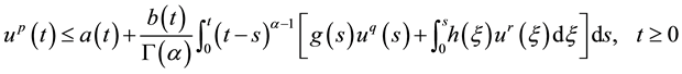
In this paper, combining (1) and (2), we will explore the following form of delay integral inequality
 . (3)
. (3)
Now we list some Definitions and Lemmas which can be used in this paper.
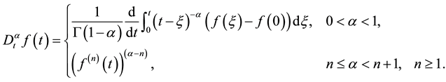
Definition 1. [6] The modified Riemann-Liouville derivative of order  is defined by
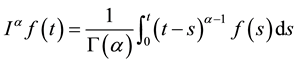
Definition 2. [6] The Riemann-Liouville fractional integral of order  on the interval
  is defined by
 .
.
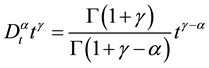
Some important properties for the modified Riemann-Liouville derivative and fractional integral are listed as follows [6] (the interval concerned below is always defined by ).
).
(1) ,
,
(2) ,
,
(3) ,
,
(4) ,
,
(5) .
.
Lemma 1. [3] Assume that![]() ,
, ![]() , and
, and![]() , then
, then
![]() .
.
Lemma 2. [6] Let![]() ,
, ![]() ,
, ![]() ,
, ![]() be continuous functions defined on
be continuous functions defined on![]() .
.
Then for![]() ,
,
![]()
Implies
![]() .
.
2. Main Results
Theorem 1 Assume that![]() ,
, ![]() ,
, ![]() ,
, ![]() ,
, ![]() ,
, ![]() ,
, ![]() , and
, and![]() ,
, ![]() are nondecreasing functions in
are nondecreasing functions in![]() . If
. If ![]() satisfies the following form of delay integral inequality
satisfies the following form of delay integral inequality
![]() , (4)
, (4)
with the initial condition
![]() ,
,
![]() (5)
(5)
where![]() ,
, ![]() ,
, ![]() ,
, ![]() ,
, ![]() ,
, ![]() ,
, ![]() ,
, ![]() are constants,
are constants, ![]() ,
, ![]() ,
,
![]() and
and![]() , then we have
, then we have
![]() (6)
(6)
for any![]() , where
, where
![]()
Proof. Fix![]() , let
, let
![]() , (7)
, (7)
![]() ,
,
Since![]() ,
, ![]() ,
, ![]() ,
, ![]() ,
, ![]() ,
, ![]() ,
, ![]() , there’s exist a constant
, there’s exist a constant![]() , such that
, such that
![]() ,
,
and ![]() is convergence integral,
is convergence integral,
so we have
![]()
we have ![]() is a nonnegative and nondecreasing. From (4) and (7) we get
is a nonnegative and nondecreasing. From (4) and (7) we get
![]() , (8)
, (8)
and
![]() . (9)
. (9)
So for ![]() with
with![]() , we have
, we have
![]() , (10)
, (10)
for ![]() with
with![]() , we have
, we have
![]() . (11)
. (11)
Combining (10) and (11), we obtain
![]() , (12)
, (12)
From (8), (9) and (12) we get
![]() , (13)
, (13)
By Lemma 1 we have
![]() (14)
(14)
Since![]() ,
, ![]() ,
, ![]() are continuous and there exists a constant
are continuous and there exists a constant ![]() satisfies
satisfies
![]()
for![]() , where
, where![]() . Then we get
. Then we get
![]() ,
,
so we have
![]() , (15)
, (15)
Using Lemma 2 to (14) we get
![]() (16)
(16)
Letting ![]() in (16) and considering
in (16) and considering ![]() is arbitary, after substituting
is arbitary, after substituting ![]() with
with![]() , we get
, we get
![]() (17)
(17)
Combining (8) and (17), we get (6).
Remark 1. Assume![]() , then the inequalities in Theorem 1 reduce to Lemma 5 in [6] .
, then the inequalities in Theorem 1 reduce to Lemma 5 in [6] .
Theorem 2. Assume that![]() ,
, ![]() ,
, ![]() ,
, ![]() ,
, ![]() ,
, ![]() ,
, ![]() ,
, ![]() are defined as in Theorem 1. If
are defined as in Theorem 1. If ![]() satisfies the following form of integral inequality,
satisfies the following form of integral inequality,
![]() , (18)
, (18)
where![]() ,
, ![]() ,
, ![]() ,
, ![]() are constants and
are constants and ![]() satisfy
satisfy
![]() , (19)
, (19)
with the condition (5) in Theorem 1, then we have
![]() , (20)
, (20)
where
![]()
![]() .
.
Proof. Let
![]() , (21)
, (21)
Since ![]() are nonegative functions,
are nonegative functions, ![]() is also nonegative and nondecreasing func- tion, in addition, there exists a constant
is also nonegative and nondecreasing func- tion, in addition, there exists a constant ![]() satisfying
satisfying
![]()
for![]() , where
, where![]() . Then we get
. Then we get
![]() ,
,
so we can get![]() . From (18) we have
. From (18) we have
![]() , (22)
, (22)
and
![]() . (23)
. (23)
By Lemma 1 we get for any![]() ,
,
![]() . (24)
. (24)
Proceeding the similar proof of Theorem 3 in [3] , we can get
![]() . (25)
. (25)
From (23), (24), (25) and condition (19) we have
![]() (26)
(26)
By Lemma 2 we have
![]() . (27)
. (27)
Combining (22) and (27), (20) can be obtained subsequently.
Theorem 3. Assume that![]() ,
, ![]() ,
, ![]() ,
, ![]() ,
, ![]() ,
, ![]() and
and ![]() is nondecreasing with
is nondecreasing with ![]() for
for![]() . If
. If ![]() satisfies
satisfies
![]() , (28)
, (28)
then
![]() , (29)
, (29)
where
![]() .
.
Proof. Let
![]() ,
,
then we get
![]() . (30)
. (30)
Since ![]() are both continuous functions,
are both continuous functions, ![]() is continuous and there exists a con-
is continuous and there exists a con-
stant ![]() satisfying
satisfying ![]() for
for![]() , where
, where![]() . Then we get
. Then we get
![]() ,
,
so we get ![]() and
and
![]()
By Lemma 2 we have
![]() . (31)
. (31)
Combining (30) and (31), we get (29).
Remark 2. Considering ![]() in Theorem 3, proceeding the similar proof of Theorem 3, we can get
in Theorem 3, proceeding the similar proof of Theorem 3, we can get
![]() .
.
Theorem 4. Assume that![]() ,
, ![]() ,
, ![]() ,
, ![]() ,
, ![]() and
and ![]() is nonde- creasing with
is nonde- creasing with ![]() for
for![]() ,
, ![]() with
with![]() . If
. If ![]() satisfies the following form of delay integral inequality
satisfies the following form of delay integral inequality
![]() , (32)
, (32)
then
![]() , (33)
, (33)
where
![]() ,
,
![]() .
.
Proof. Let
![]() ,
,
then we get
![]() , (34)
, (34)
The assumptions on ![]() and
and ![]() imply that
imply that ![]() is nondecreasing and there exists a constant
is nondecreasing and there exists a constant
![]() satisfying
satisfying ![]() for
for![]() , where
, where![]() .
.
Then we get
![]() ,
,
so we have![]() . For
. For![]() , we have
, we have
![]() ,
,
and
![]() (35)
(35)
Using Lemma 4 to (35), we can get
![]() . (36)
. (36)
Combining (34) and (36), we get (33).
Remark 3. Considering ![]() and
and ![]() in Theorem 4, we can get Remark 2.
in Theorem 4, we can get Remark 2.
3. Applications
In this section, we will show that the inequalities established above are useful in the research concerning the boundness, uniqueness and continuous dependence on the initial value for solutions to fractional differential equations.
3.1. Consider the Following Fractional Differential Equation
![]() ,
,
![]() . (37)
. (37)
with the condition
![]() ,
,
![]() , (38)
, (38)
where![]() ,
, ![]() is a constant,
is a constant, ![]() ,
, ![]() ,
, ![]() ,
,
And
![]() ,
,
Example 1. Assume that ![]() satisfies
satisfies
![]() , (39)
, (39)
where ![]() are nonnegative continuous functions on
are nonnegative continuous functions on![]() , then we have the following estimate for
, then we have the following estimate for![]() ,
,
![]() (40)
(40)
where
![]() .
.
Proof. By Equation (37), we have
![]() . (41)
. (41)
By (39) and (41) we can get
![]() (42)
(42)
With a suitable application of Theorems 1 to (42) (with![]() ,
, ![]() ,
, ![]() ,
, ![]() ,
,![]() ), we can obtain the desired result. This complete the proof of Example 1.
), we can obtain the desired result. This complete the proof of Example 1.
Example 2. Assume that
![]() , (43)
, (43)
where ![]() are nonnegative continuous functions defined
are nonnegative continuous functions defined![]() ,
, ![]() is the quotient of two odd num- bers. Equation (37) has a unique solution.
is the quotient of two odd num- bers. Equation (37) has a unique solution.
Proof. Suppose ![]() are two solutions of Equation (37), then we have
are two solutions of Equation (37), then we have
![]()
Furthermore,
![]()
which implies
![]() (44)
(44)
Through a suitable application of Theorem 1 to (44) (with![]() ,
, ![]() ,
,![]() ), we can obtain
), we can obtain
![]() ,
,
which implies![]() . So Equation (37) has a unique solution.
. So Equation (37) has a unique solution.
Example 3. Suppose that ![]() is the solution of (37) and
is the solution of (37) and ![]() be the solution of the following fractional integral equation,
be the solution of the following fractional integral equation,
![]() ,
,
![]() . (45)
. (45)
If ![]() satisfies the condition (43), then the solution of Equation (37) depends on the initial value
satisfies the condition (43), then the solution of Equation (37) depends on the initial value ![]() continuously.
continuously.
Proof. By Equation (45), we have
![]() , (46)
, (46)
so we get
![]()
Furthermore
![]() (47)
(47)
Apply Theorem 1 to (47) (with![]() ,
, ![]() ,
, ![]() ,
,![]() ), we get
), we get
![]() ,
,
where![]() . This gives that the solutions of Equation (37) depends on the initial value
. This gives that the solutions of Equation (37) depends on the initial value ![]() continuously.
continuously.
3.2. Consider the Following Fractional Differential Equation
![]() ,
,
![]() . (48)
. (48)
Example 4. Assume that ![]() is a solution of Equation (48), then
is a solution of Equation (48), then ![]() is bounded.
is bounded.
Proof. By Equation (48) we can get
![]() . (49)
. (49)
with a suitable application of Theorem 3 to (49) (with![]() ,
, ![]() ,
, ![]() ,
, ![]() ,
, ![]() for
for![]() ,
, ![]() ,
,![]() ), we have
), we have
![]()
where we used![]() . This complete the proof of Example 4.
. This complete the proof of Example 4.
Example 5. If ![]() is a solution of (48), then it has a unique solution.
is a solution of (48), then it has a unique solution.
Proof. Suppose ![]() are two solutions of Equation (48), then we have
are two solutions of Equation (48), then we have
![]()
Furthermore,
![]() ,
,
which implies
![]() . (50)
. (50)
With a suitable application of 3 to (50) (with![]() ,
, ![]() ,
, ![]() ,
, ![]() ,
, ![]() ,
, ![]() for
for![]() ), we can obtain
), we can obtain
![]() ,
,
which implies![]() . So Equation (48) has a unique solution.
. So Equation (48) has a unique solution.
Example 6. Suppose that ![]() is the solution of (48) and
is the solution of (48) and ![]() is the solution of the following fractional integral equation,
is the solution of the following fractional integral equation,
![]() ,
,
![]() . (51)
. (51)
Then all the solutions of Equation (48) depend on the initial value ![]() continuously.
continuously.
Proof. By Equation (51), we have
![]() ,
,
so we get
![]()
Furthermore
![]() . (52)
. (52)
Apply Theorem 3 to (52) (with![]() ,
, ![]() ,
, ![]() ,
, ![]() ,
, ![]() for
for![]() ,
,
![]() ,
,![]() ), we get
), we get
![]() (53)
(53)
where we use the fact that ![]()
This gives that ![]() depends on the initial value
depends on the initial value ![]() continuously.
continuously.
Acknowledgements
We thank the Editor and the referee for their comments. This work is supported by National Science Foundation of China (11171178 and 11271225).