HAC-Robust Measurement of the Duration of a Trendless Subsample in a Global Climate Time Series ()
1. Introduction
The 2013 report of the Intergovernmental Panel on Climate Change drew attention to a pause, or “hiatus” in what appears otherwise to be a long upward trend in globally-averaged temperatures ([1] Ch. 9). Figure 1 shows the HadCRUT4 combined land and ocean surface temperature series over the 1850-2014 interval [2] . The data are shown in the form of ˚C “anomalies” or deviations from local averages. The underlying trend is clearly up-

Figure 1. Globally-averaged HadCRUT4 surface temperature anomalies, January 1850 to April 2014. Dark line is lowess smoothed with bandwidth parameter = 0.09.
ward over the 20th century, but a leveling off at the end is visible. Figure 2 shows the lower troposphere (LT) series from the University of Alabama-Huntsville method (denoted UAH, [3] ) and Figure 3 shows the LT series using the RSS method of [4] . These observations run from January 1979 to April 2014 and show a similar leveling-off over the ending segment.
The IPCC does not estimate the duration of the hiatus, but it is typically regarded as having extended for 15 to 20 years. While the HadCRUT4 record clearly shows numerous pauses and dips amid the overall upward trend, the ending hiatus is of particular note because climate models project continuing warming over the period. Since 1990, atmospheric carbon dioxide levels rose from 354 ppm to just under 400 ppm, a 13% increase. [1] reported that of the 114 model simulations over the 15-year interval 1998 to 2012, 111 predicted warming. [5] showed a similar mismatch in comparisons over a twenty year time scale, with most models predicting 0.2˚C - 0.4˚C/ decade warming. Hence there is a need to address two questions: 1) how should the duration of the hiatus be measured? 2) Is it long enough to indicate a potential inconsistency between observations and models? This paper focuses solely on the first question. For an approach to the second, see [6] .
Several considerations need to be addressed in order for a duration measure to be robust. Consider a basic trend model
 (1)
(1)
in which yt is assumed to be trend-stationary (in other words, does not contain a unit root), a and b are coefficients to be estimated, t is a linear trend spanning  and et is a covariance-stationary residual which may be described as autocorrelated or persistent to unknown dimensions. A series with a positive trend is one for which
 , (2)
, (2)
where  is the (
 ) confidence interval around
 . An end-of-sample pause in the upward trend is defined using the duration parameter J, defined such that
 (3)
(3)
in other words the maximum length subset of the final observations of the series  such that the (
 ) confidence interval around the trend term contains zero. Throughout this paper we use
  and hence a 95% confidence interval. Framed this way, two criteria can be set down to ensure robustness.
a) The confidence interval must be heteroskedasticity and autocorrelation (HAC) robust. While the IPCC itself typically uses a simple AR1 process to model residuals, there is empirical evidence that the error processes exhibit higher-order autocorrelation and long term persistence [6] -[8] . Tests of the series used herein all showed evidence of higher than first-order autocorrelation. Hence the estimator must be valid for longer memory structures.
b) The longer is T, the more likely it is possible to find a single spurious value J that satisfies Equation (3)

Table 1 Results for sequential tests of surface trend hiatus. J: length of pause being considered. Start year: implied beginning year of pause. CI Lower Bound and Upper Bound: 95% confidence interval limits from Equation (8). Estimated Global Trend: . VF on Global Trend: VF from Equation (9) applied to HadCRUT4 series. The 5% critical value is 41.53. VF on test SH = NH = 0: VF test score from Equation (8) on null hypothesis
 , where the two series are the NH and SH averages from HadCRUT4. The 5% critical value is 40.68.

Figure 2. Globally-averaged UAH lower troposphere temperature anomalies, January 1979 to April 2014. Dark line is lowess smoothed with bandwidth parameter = 0.11.
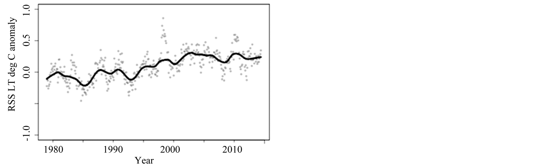
Figure 3. Globally-averaged RSS lower troposphere temperature anomalies, January 1979 to April 2014. Dark line is lowess smoothed with bandwidth parameter = 0.11.
even if, for all other values of J, the trend is significant. To avoid cherry-picking J, if it really marks the beginning of a pause in the trend, rather than being simply an artefact of the pseudo-cyclical behavior of persistent residuals, we require that condition (3) be observed at every point in the interval .
.
A further condition can be added for the specific case studied here, namely globally-averaged surface temperatures, that there ought to be spatial consistency, namely c) conditions (3), (a) and (b) ought to hold jointly in both the Northern and Southern Hemispheres, since a pause in only one but not both would not be truly global, even if it caused the average of the two series to have an insignificant trend.
Combining (a)-(c) yields the following definition of hiatus length:
DEFINITION: A globally-averaged temperature series of length T with an upward trend coefficient b has a robust end-of-sample pause of length  if, for every interval beginning at
  and ending at time T, where m is the minimum-length duration of interest,
  , the (
 ) confidence interval
  is HAC-robust, and the value of
  computed for both the Northern and Southern Hemispheres equals or exceeds that for the globe as a whole.
I apply this definition to the HadCRUT4, UAH and RSS series, obtaining hiatus durations of, respectively, 19, 16 and 26 years respectively. Were one to use an AR1 method the estimated durations would be 14, 14 and 20 years respectively.
2. Application of Hiatus Definition to Surface and Tropospheric Temperature Data
2.1. The VF Test and HAC-Robust Confidence Intervals
To address condition (a) I apply the HAC-robust trend confidence interval estimator of [9] (hereafter VF). HAC methods are very common in econometrics and have recently been applied in climatology, see [6] . The VF approach falls in the class of non-parametric HAC estimators, but avoids the problem of bandwidth selection by setting it equal to the sample size T. The resulting estimator exhibits very little size distortion in comparison to other HAC estimators using limited bandwidth, while maintaining comparable power levels. However, the estimator converges to a non-standard distribution so the critical values must either be simulated or computed using the bootstrap method. In the case of straightforward trend estimation, as in the current application, critical values are available in VF.
The trend coefficient is estimated on monthly data using OLS. The full derivation of the variance-covariance estimator, including asymptotics, is available in VF, and I will only explain the computational steps here. Since we will apply the test not only to the global series but also jointly to hemispheric trends, I will present it for the multivariate case.
A multivariate trend model is written
 . (4)
. (4)
where , the number of time series for which trends are to be measured and tested. Denote
 and
and . We are interested in testing null hypotheses of the form
 . (5)
. (5)
against alternatives  where R and r are known restriction matrices of dimension q × N and q × 1 respectively, where q denotes the number of restrictions being tested. The matrix R is assumed to have full row rank. Robust tests of
  need to account for correlation across time, correlation across series, and conditional heteroskedasticity as summarized by the long run variance of
 . This is defined as
 . (6)
. (6)
where  is the matrix autocovariance function of et. The VF statistic is constructed using the following estimator of Ω:
 . (7)
. (7)
where . This is the Bartlett kernel nonparametric estimator of Ω using a bandwidth (truncation lag) equal to the sample size. The VF statistic for testing
  is given by
 . (8)
. (8)
where  are the residuals from regressing the trend t on a constant. Equation (7) was originally proposed by [10] although in the different but computationally identical form:
 . (9)
. (9)
where . See [11] for proof of the equivalence between (6) and (9).
In the univariate case (q = 1), the square root of (7) can be interpreted as a t-type statistic and critical values are tabulated in VF. By treating the denominator as the robust standard error term , a HAC-robust 95% confidence interval can be constructed
 . (10)
where the 0.025 critical value  is, from VF, 6.482. The confidence interval given by Equation (10) is robust to all forms of autocorrelation up to but not including a unit root. All the data series used herein were tested using a Dickey-Fuller test and in every case the unit root hypothesis was rejected.
The AR1 case is handled differently, using the Bartlett approximation of [12] , in which the lag-one AR coefficient r is estimated using the Cochrane-Orcutt iterative method, then the standard errors are scaled up by the factor . This yields a valid approximation to the long-run variance only if the error terms are AR1. However the data series used herein are known to exhibit higher-order autocorrelation (see, e.g. [6] -[8] ) so the AR1 approach will likely lead to over-rejections of the null, which in this case implies under-estimation of
 .
.
2.2. Results for the HadCRUT4 Series
Table 1 presents the surface results. The data are monthly but we only consider annual increments for J, and only for durations of more than m = 5 years, as failure to reject the null of no trend in the vicinity of the end of the sample could, in the case of such a short interval, arise simply due to the small size of the subsample. The bolded line at J = 19, for the year 1995, shows the maximum value of J for which the lower bound of the confi
dence interval is negative, thus indicating that Equation (3) is satisfied. Looking up the column from there it can be seen that condition (b) is also satisfied. In column 7, the number shown is the VF score on the test that the separate NH and SH trends are jointly zero. The 5% critical value for the q = 2 case is 40.68, which is only exceeded at J = 23, therefore the additional condition (c) is also met in this case. Hence, for the surface HadCRUT4 data, .
.
Figure 4 shows these results in graphical form. It is clear that the confidence intervals widen at the end of the sample as J increases and the number of degrees of freedom decline, but not before first shrinking somewhat, indicating that at the computed value of  the number of degrees of freedom is not the limiting factor on the size of the confidence interval.
2.3. Results for the UAH and RSS Series
Table 2 and Table 3 present the UAH and RSS series, respectively. For UAH, the bolded line at J = 16, corresponding to the year 1998, shows the maximum value of J for which the lower bound of the confidence interval
Table 2 . Results for sequential tests of UAH trend hiatus. J: length of pause being considered. Start year: implied beginning year of pause. CI Lower Bound and Upper Bound: 95% confidence interval limits from Equation (8). Estimated Global Trend: . VF on Global Trend: VF from Equation (9) applied to UAH series. The 5% critical value is 41.53. VF on test SH = NH = 0: VF test score from Equation (8) on null hypothesis
 , where the two series are the NH and SH averages from UAH. The 5% critical value is 40.68.
Table 3. Results for sequential tests of RSS trend hiatus. J: length of pause being considered. Start year: implied beginning year of pause. CI Lower Bound and Upper Bound: 95% confidence interval limits from Equation (8). Estimated Global Trend: . VF on Global Trend: VF from Equation (9) applied to RSS series. The 5% critical value is 41.53. VF on test SH = NH = 0: VF test score from Equation (8) on null hypothesis
 , where the two series are the NH and SH averages from RSS. The 5% critical value is 40.68.

Figure 4. Trend magnitudes (black dots) and 95% robust confidence intervals (solid lines) around trend in HadCRUT4 global series from start date indicated to April 2014.

Figure 5. Trend magnitudes (black dots) and 95% robust confidence intervals (solid lines) around trend in UAH lower troposphere series from start date indicated to April 2014.
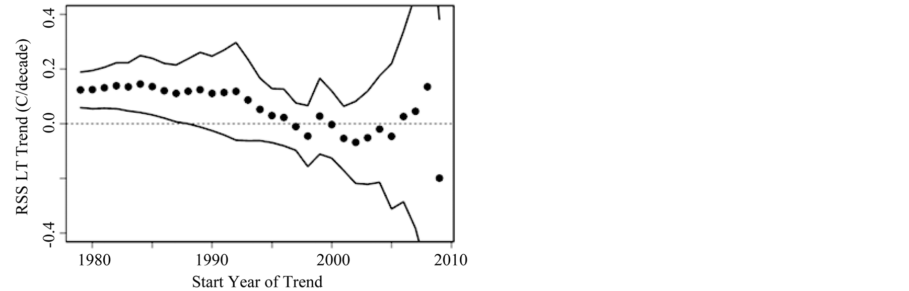
Figure 6. Trend magnitudes (black dots) and 95% robust confidence intervals (solid lines) around trend in RSS lower troposphere series from start date indicated to April 2014.
is negative. Looking up the column from there it can be seen that condition (b) is also satisfied. In column 7, the VF score on the joint NH and SH trend tests only exceed 40.68 at J = 19, therefore the additional condition (c) is also met in this case. Hence, for the lower troposphere UAH data, . Figure 5 shows the UAH results in graphical form. For the RSS results, comparable examination yields
 , corresponding to a start date at 1988. The results are shown in Figure 6.
3. Conclusion
I propose a robust definition for the length of the pause in the warming trend over the closing subsample of surface and lower tropospheric data sets. The length term  is defined as the maximum duration J for which a valid (HAC-robust) trend confidence interval contains zero for every subsample beginning at J and ending at
  where m is the shortest duration of interest. This definition was applied to surface and lower tropospheric temperature series, adding in the requirement that the southern and northern hemispheric data must yield an identical or larger value of
 . In the surface data we compute a hiatus length of 19 years, and in the lower tropospheric data we compute a hiatus length of 16 years in the UAH series and 26 years in the RSS series.
  estimates based on an AR1 estimator are lower but likely incorrect since higher-order autocorrelation exists in the data. Overall this analysis confirms the point raised in the IPCC report [1] regarding the existence of the hiatus and adds more precision to the understanding of its length.