The Solution of Nonlinear Equations via the Method of Hurwitz-Radon Matrices ()
1. Introduction
A significant problem in computer vision and image analysis [1] is to solve any nonlinear equation . This means the issue of approximation
  in equation
  where
where . Two-dimensional data can be treated as points on the curve. Many numerical methods for nonlinear equations are known as iterative methods: bisection, regula falsi, Newton’s method (also called as the Newton-Raphson method), Steffensen’s method, Brent’s method, Broyden’s method, fixed-point iterations, inverse interpolation and the secant method [2] . These methods can be used for any function, but sometimes there are troubles. For example in Newton’s method we may found difficulties in calculating derivative of a function or troubles with bad starting point of iteration. Generally iterative methods need many assumptions about function (monotonicity, convexity, derivative, starting point). Some methods are used only for polynomials (Muller’s, Laguerre’s, Bairstow’s, Jenkins-Traub’s methods). Nonlinear systems are still opened for researchers [3] .
This paper is dealing with novel method of root’s approximation by using a family of Hurwitz-Radon matrices. Method of Hurwitz-Radon Matrices (MHR) does not need any assumption about function. The only information about curve is the set of at least five interpolation nodes and a zero of the function between two of them. Proposed method of Hurwitz-Radon Matrices (MHR) is used in data interpolation and then calculations to solve the nonlinear equation are introduced. MHR connects two significant problems in mathematics and computer sciences: interpolation of the function and the solution of nonlinear equation [4] . MHR method uses two-dimensional data for knowledge representation [5] and computational foundations [6] . Also medicine [7] , industry and manufacturing are looking for the methods connected with geometry of the curves [8] . So suitable data representation and precise solving of any equation [9] are the key factors in many applications of artificial intelligence and numerical methods [10] .
2. Assumptions for the Solution
Each nonlinear equation is represented by  and succeeding points
  of function
  (interpolation nodes) as follows in proposed MHR method:
1. first node  and last node
  must fulfill a condition
 ;
;
2. at least three nodes , for example equidistant between first and last node, have to be calculated (for
 ) if MHR method is used with matrices of dimension
 .
.
Condition 1 is well known in numerical methods for existing a zero of the function. Condition 2 is connected with important features of MHR method: MHR version with matrices of dimension  (called MHR-2) needs at least five nodes (for
 ), MHR version with matrices of dimension
  (called MHR-4) needs at least nine nodes (for
 ) and MHR version with matrices of dimension
  (called MHR-8) needs at least 17 nodes (for
 ).
).
Figure 1 presents the graph of function  with nodes: first
 and last
 . All five nodes are applied in MHR calculations, but a root of function is searched only between nodes
  and
and . The approximation of a zero point of the function is possible using novel MHR method.
3. Reconstruction of the Graph Points
The key question exists in many branches of science: is it possible to find a method of nonlinear equation solution without iterations of numerical methods [11] ? This paper aims at giving the positive answer to this question. Method of Hurwitz-Radon Matrices (MHR), described in this paper, is computing points between two successive nodes for searching a root of the function. The curve or function in MHR method is parameterized for real number  in the range of two successive interpolation nodes.

Figure 1. Five nodes of function and a root between first and second node (MS Excel graph).
3.1. The Operator of Hurwitz-Radon
Adolf Hurwitz (1859-1919) and Johann Radon (1887-1956) published the papers about specific class of matrices in 1923, working on the problem of quadratic forms. Matrices ,
,  satisfying

are called a family of Hurwitz-Radon matrices. A family of Hurwitz-Radon (HR) matrices has important features [12] : HR matrices are skew-symmetric  and reverse matrices are easy to find
 . Only for dimension
  or 8 the family of HR matrices consists of
  matrices. For
  there is one matrix:

For  there are three HR matrices with integer entries:

For  we have seven HR matrices with elements 0, ±1. So far HR matrices are applied in electronics [13] : in Space-Time Block Coding (STBC) and orthogonal design [14] , also in signal processing [15] and Hamiltonian Neural Nets [16] .
If one curve is described by a set of following points  then HR matrices combined with the identity matrix IN are used to build the orthogonal and discrete Hurwitz-Radon Operator (OHR). For nodes
  and
and  OHR
OHR  of dimension
  is constructed:
 . (1)
. (1)
For nodes  and
and  OHR of dimension
  is constructed:
 (2)
(2)
where

For nodes  and
and  OHR of dimension
  is built [17] similarly as (1) and (2):
 (3)
(3)
where
 (4)
(4)
The components of the vector , appearing in the matrix
  (3), are defined by (4) in the similar way to (1) and (2) but in terms of the coordinates of the above 8 nodes. Note that OHR operators
  (1)-(3) satisfy the condition of interpolation
 (5)
(5)
For  or 8.
or 8.
3.2. Points Interpolation by MHR
Key question looks as follows: how can we compute coordinates of points settled between the interpolation nodes [18] ? The answer is connected with novel MHR method [19] . On a segment of a line every number “ ” situated between “
 ” and “
 ” is described by a linear (convex) combination
  for
for
 (6)
(6)
The average OHR operator  of dimension
  or 8 is constructed as follows:
 (7)
(7)
with the operator  built (1)-(3) by “odd” nodes
  and
and  built (1)-(3) by “even” nodes
 . Having the operator
  it is possible to reconstruct the second coordinates of points
  in terms of the vector
  defined with
 (8)
(8)
as . The required formula is similar to (5):
 (9)
(9)
in which components of vector  give the second coordinate of the points
  corresponding to the first coordinate, given in terms of components of the vector
 .
.
Calculations of unknown coordinates for curve points using (6)-(9) are called by author the method of Hurwitz-Radon Matrices (MHR) [20] . Here is the application of MHR method (Figure 2) for function  with nodes as Figure 1 and computed 99 points between each pair of nodes
 .
.
Solving the equation  via MHR interpolation, as it was said under Figure 1, we search a root of the function only between nodes
  and
and . Points calculated between other pairs of nodes are useless in the process of root approximation and they don’t have to be computed. Considering calculated points between nodes
  and
and , second coordinate is near zero at
 . Solution of equation
  via MHR-2 method is approximated by
 . True value is
 .
.
The same equation for nodes  and
and , solved by MHR-2, gives better result
 . So shorter distance between first and last node is of course
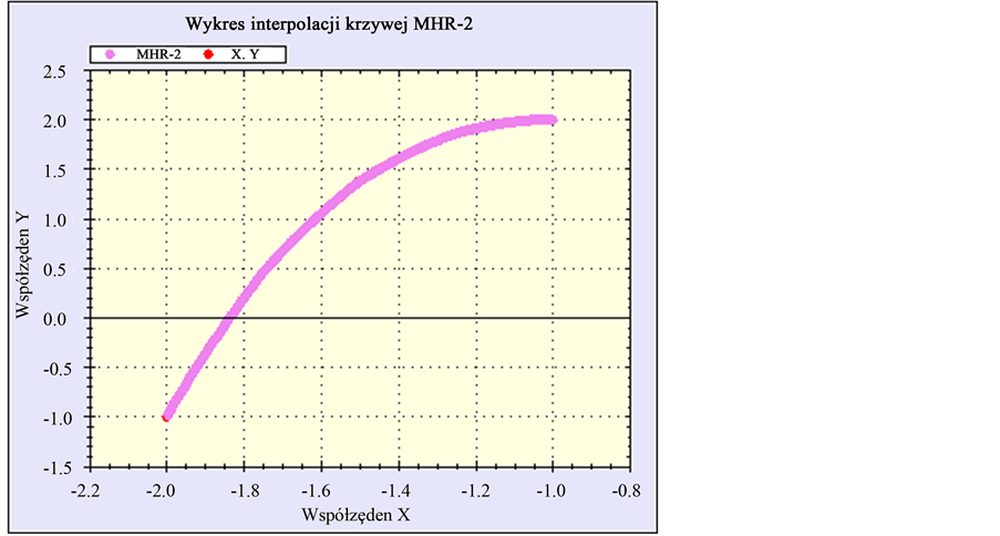
Figure 2. Function 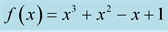 with 396 interpolated points using MHR-2 method.
very important feature.
4. Nonlinear Equations Solved via MHR
Example 1 MHR calculations are done for function  with nodes:
  and
and . So a root of this function is situated between 3rd and 4th node. MHR-2 interpolation gives the graph of function (Figure 3):
Considering points between nodes  and
and , coordinate y is near zero at
 . Solution of equation
  via MHR method is approximated by
 . True value is hardly approximated (even for MathCad) by
 .
.
Example 2 MHR calculations are completed for function  with nodes:
  and
and . So a zero of this function is situated between 2nd and 3rd node. MHR-2 computes the graph of function (Figure 4).
Considering points between nodes  and
and , coordinate y is near zero at
 . Solution of equation
  via MHR-2 is approximated by
 . The only one real solution of this equation is
 .
.
Now MHR calculations are done for the same equation  with seven nodes between
  and
and  for
for  and 1. The solution is approximated by MHR-4 method with nine nodes. MHR-4 interpolation gives the graph of function (Figure 5).
Considering points between nodes and
and , coordinate y is near zero at
 . Solution of equation
  via MHR-4 is approximated by
 . This is better result than MHR-2: greater number of nodes (with the same distance between first and last) means better approximation. And seventeen nodes in MHR-8 guarantee more precise results then MHR-4.
Example 3 MHR calculations are done for equation  with nodes:
  and
and . MHR-2 gives the graph of function (Figure 6).
Considering points between nodes  and
and , second coordinate is near zero at
 . Solution of equation
  via MHR-2 method is approximated by
 . Pre-
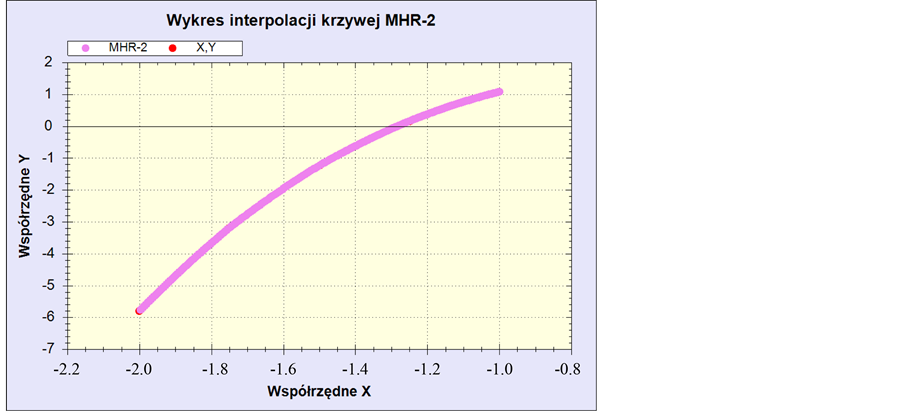
Figure 3. Function  with 396 interpolated points using MHR-2.

Figure 4. Function  with 396 interpolated points using MHR-2.
cise solution  is approximated by 1.585.
Interpolated values, calculated by MHR method, are applied in the process of solving the nonlinear equations. Shorter distance between first and last node or greater number of nodes guarantee better approximation. Approximated solutions of nonlinear equations are used in many branches of computer sciences. MHR joins two important problems: interpolation of the function with the solution of nonlinear equation.
5. Conclusions
The method of Hurwitz-Radon Matrices leads to curve interpolation [21] and approximation of nonlinear equation solution depending on the number and location of nodes. No characteristic features of function is important
Figure 5. Function 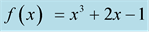 with interpolated points using MHR- 4 method with 9 nodes.
Figure 6. Function  with 396 interpolated points using MHR- 2 method with 5 nodes.
in MHR method: polynomial or not, monotonicity, convexity, derivative, starting point. These features are very significant for iterative numerical methods. MHR method gives the possibility of reconstruction a curve and searching for a root of the function. The only condition is to have a set of nodes according to assumptions in MHR method. The features of MHR method: accuracy of the equation solution depends on the number of nodes and the distance between first and last node (MHR-4 is more precise than MHR-2 and MHR-8 is more precise than MHR-4); interpolation of a curve consists of  points is connected with the computational cost of rank
 ; MHR is a well-conditioned method (orthogonal matrices); MHR is not an affine interpolation [22] .
Future works are connected with: computing the interpolation error, implementation of MHR in object recognition [23] , MHR extrapolation method [24] and curve parameterization [25] .