Price and Income Elasticities of Gasoline Demand in Iran: Using Static, ECM, and Dynamic Models in Short, Intermediate, and Long Run ()
1. Introduction
Since the two oil price shocks in 1970 and 1973, interest in the study of oil products demand has increased considerably, especially on gasoline [1] [2] . These studies assessed the economical, environmental, and political impacts by evaluating the key elements of gasoline demand. Despite deeply concerning of oil producing countries with the international oil products demand, they pay little attention to the domestic demand of the products [3] . For example, gasoline consumption is a serious crisis in Iran which increased considerably until 2006 [4] , causing great threats. The consumption of gasoline, as a subsidized good, is very high in Iran because of the low price which is determined by the government [5] .
High gasoline consumption is a serious crisis in Iran, posing economically, politically, and environmentally threats [6] . The gasoline consumption has outnumbered the production level leading to import gasoline. Not only the decreasing balance of payments, economically, but also increasing energy dependency, politically, has threatened the country. As a negative externality, it has resulted in environmental pollution, reducing social welfare [5] . These threats have raised the concerns with the high gasoline consumption.
Due to the great threats, policy makers have planned some strategies to turn down the consumption. For example, Iranian government has forced up the gasoline price noticeably by removing the subsidy in 2007 [6] . The policy can reduce the consumption but it is not clear whether it is effective enough in the reduction or ineffective.
The main objective of this paper is to evaluate the price and income elasticities of gasoline demand in Iran. It shows whether the price policy, pursued by the Iranian government, can decrease the gasoline consumption sufficiently or not. If the gasoline consumption responds insufficiently to the price policy, the governors should choose other alternatives. So estimating price and income elasticities of gasoline demand paves the way to make the right decision.
2. Literature Review
There is a large number of studies on gasoline demand with different methods. Table 1 displays different studies and surveys on price and income elasticities of gasoline demand. In three different decades, Dahl (2012), Dahl and Sterner (1991), and Espey (1998) have categorized the important studies, according to the models and estimates [7] -[9] . So a review of the surveys improves an outlook on the subject, before dealing with studies in details.

Table 1. Previous studies and surveys on price and income elasticities of gasoline demand.
aShort-Run (SR) and Long-Run (LR); bAveragely.
Dahl and Sterner (1991) have reviewed 97 studies on gasoline demand, the most recent one published in 1988. Despite using different estimation methods, all of the studies have estimated real price and real income as explanatory variables. Due to the vastly various models in the studies, they broke the models into ten “distinct groups” which show nearly unique results. They claim that gasoline demand is mostly inelastic with respect to price and income. Moreover, they argue that correlating the first model with the second models of the ten groups resulted in intermediate run elasticities [8] . There are more recent reviews like this survey.
Espey (1998) has surveyed 101 studies on gasoline demand, made within 1966-1997 with data period from 1929 to 1993. According to the survey, functional forms and countries are very different but all of them use real price and real income as explanatory variables. Due to the vast range of elasticities in the previous studies, he classified the short run and long run estimates into several groups [9] . Likewise, Dahl (2012) has classified the gasoline demand price and income elasticities of the previous studies with static models into many groups [7] . Overall, the most frequent elasticities imply that gasoline demand is maily inelastic with respect to price and income both in Espey (1998) and in Dahl (2012) [7] [9] . Meta-analyses, like Dahl (2012), Dahl and Sterner (1991), and Espey (1998), deal with the issue as a whole [7] -[9] .
There are many surveys which cover the literature generally but reviewing some studies expresses a more detailed attitude of developed countries. Baranzini and Weber (2013) have estimated the price and income elasticities of gasoline demand in Switzerland, employing cointegrating equation and Error Correction Model (ECM). They showed that it is inelastic with respect to both price and income, over the short run and long run. The adjustment velocity is low, at −0.27, meaning a slow rate of adjustment to the long run equilibrium [10] . Wadud et al. (2009) have obtained the elasticities in USA with cointegration technique. They are inelastic too, just like the last study [11] .
Sene (2012), Akinboade et al. (2008), and Ramanathan (1999) concentrated on some developing countries [5] [12] [13] . Sene (2012) has estimated short run and long run price and income elasticities in Senegal, using log linear model. He found that the gasoline demand is inelastic because oil products do not have close substitutes [12] . Akinboade et al. (2008) estimated price and income elasticities of gasoline demand with Autoregressive Distributed Lag Model (ARDL) in South Africa. They showed that the gasoline demand is inelastic in the countries [14] . Ramanathan (1999) has employed cointegrating equation and Error Correction Model (ECM) to estimate the elasticities of gasoline demand in India through two intervals, short run and long run, as well as the adjustment velocity. Although the estimated gasoline demand is income elastic, it is price inelastic in both the spans. The adjustment velocity is low, at 28%, around that of Baranzini and Weber (2013) [10] [13] . Eltony and Al-Mutairi (1995) have argued that gasoline demand is price and income inelastic in Kuwait, as a developing and oil producing country [15] .
Some studies focus on oil producing countries like Iran which is in gasoline consumption crisis [6] . Ahmadian et al. (2007) have claimed that the gasoline consumption is evidently high in Iran, caused by the low price of gasoline, which reduces the social welfare [5] .
3. Models
The elasticities are estimated over three intervals, short run, intermediate run, and long run in Iran during 1976- 2010, putting the estimates of Error Correction Model (ECM), static model, and dynamic model in an increasing order, respectively. Cointegration technique is used for estimation of the static model and then Error Correction Model (ECM) is employed to estimate the “adjustment velocity” [16] . After the dynamic model estimation, the results of the three models are compared with each other in order to derive the elasticities over the three intervals [8] .
3.1. Static Model
According to the previous studies, a static model [8] , also referred to as “log linear model” [10] , with cointegration technique [13] is employed to measure the price and income elasticities of gasoline demand which is as follows:
 (1)
(1)
where Ln is the natural logarithm, G is the gasoline demand, P is the real gasoline price, Y is the income, u is the residual term with usual classical characteristics  [17] , and t is year. Furthermore,
  is intercept,
  is the long run price elasticity, and
  is the long run income elasticity.
On the basis of Engel-Granger (1987) approach, a cointegrating regression signalizes a long run relationship among variables. Providing that all variables of a regression have the same integration degree of ρ, it will be a cointegrating regression if the residual series have a less integration degree than ρ [18] . In this case, parameter  in Equation (1) is interpreted as the price elasticity of gasoline demand and
  the income elasticity [16] .
3.2. Error Correction Model (ECM)
Error Correction Model (ECM) is used for the estimation of short run elasticities of gasoline demand [13] [16] which is as follows:
 (2)
(2)
where ∆ is one degree differentiation,  is the estimated residuals in the cointegrating regression, e is the residual term,
  is intercept, and the remaining symbols were explained in the previous model. The variables with one degree of integration are stationary by differentiating once. Hence, the regression shows the short run relationship among the variables as parameter
  is the gasoline price elasticity of gasoline demand and
  is the income elasticity. Also, the coefficient
  is the adjustment velocity [16] .
3.3. Dynamic Model
A dynamic model, referred to as “the partial adjustment model” and “the lagged endogenous model” [8] , is employed to verify the results of the static model. In this way, the elasticities of gasoline demand are estimated over the three intervals. The dynamic model is as follows:
 (3)
(3)
where Gt‒1 is the lagged gasoline demand,  is the residual term,
  is intercept,
  is the short run price elasticity,
  is the short run income elasticity, and
  is the lagged gasoline demand coefficient. In this model, the long run price and income elasticities are equal to
  and
and , respectively [3] [12] .
3.4. Correlating the Estimations
Putting the estimates of Error Correction Model (ECM), static model, and dynamic models in an increasing order, price and income elasticities of gasoline demand are estimated over three intervals, short run, intermediate run, and long run in Iran during 1976-2010, respectively. The elasticities, estimated by the static model, will be interpreted as the intermediate elasticities, if they wax and wane between the short run and long run elasticities, estimated by the dynamic model [8] .
4. Data
In this study, dataset includes annual time series data from 1976 to 2010. It is derived from the economic time series database of the Economic Research and Policy Department of Iran1 (see Appendix 1) [4] . Only nominal gasoline price is from the National Iranian Oil Refining and Distribution Company2 (see Appendix 2) [19] which is divided by consumer price index (2004 = 100) so that the inflation is captured. The explanatory variable is per capita gasoline consumption and the dependent variables are real gasoline price and real per capita GDP. The real per capita GDP, as a proxy for income, is GDP at current prices in Rials of Iran, divided by the consumer price index and total population. The per capita gasoline consumption, as a proxy for gasoline demand, is gasoline consumption divided by the total population. It is measured in thousand barrels per day in the database but it is converted to liters per day3 because the nominal gasoline price is the value of per liter in Rials of Iran.
Figure 1 reveals some information about how many liters of gasoline are consumed each day in Iran within
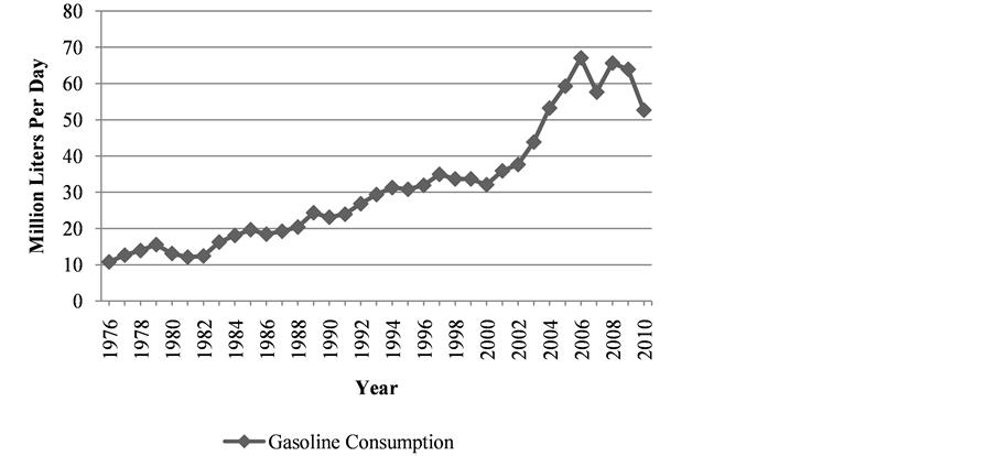
Figure 1. Gasoline consumption in million liters per day in Iran during 1976- 2010 [4] .
more than three decades, from 1976 to 2010 (see Appendix 3) [4] .
Based on the graph, the gasoline consumption moved upward during 1976-2006. Until 2002, it surged up markedly, reaching well below 40 million, quadrupling the figure in the first year. Since then, the rate of increasing accelerated within the next four years, as the gasoline consumption topped just below 70 million in 2006.
The gasoline consumption rose and fell erratically within the last four years of the span. It collapsed abruptly from in 2007 which comprised about 60 million. Although it recovered to around 65 million in 2008, it took a nosedive in the last two years which accounted for slightly over 50 million in 2010.
In summary, the gasoline consumption in Iran represents an increasing pattern from 1976 to 2010, with some fluctuations in the last four years.
Since the government paid a massive subsidy for gasoline (reaching 10.2 billion US$ in 2006), its price was low, leading to the high consumption. The high cost of subsidy payment caused the government to formulate some strategies to reduce the consumption, for example, making price policy, setting a higher environmental standard for cars, supplying an alternative fuel (CNG), and gasoline rationing [6] . These led the consumption to fall marginally within 2007-2010, except for 2008.
5. Results
Using the Augmented Dickey Fuller (ADF) unit root test, the variables are checked for stationary properties and cointegration relationship. Using Ordinary Least Squares (OLS), the cointegrating equation is regressed to estimate the price and income elasticities. Then the short run and long run elasticities are estimated by the ECM and dynamic model. The static model estimations are interpreted as the intermediate run elasticities because they are between the short run and the long run elasticities. The econometric software package Eviews version 7 and Microsoft Office Excel version 2007 are applied for the estimation.
5.1. Unit Root Test
Table 2 shows the results of the ADF tests with intercept. The estimates do not reject the null hypothesis of nonstationarity at 1% significance level but all the variables are stationary after differentiating once4. So they are integrated of the same degree, representing the evidence of cointegration.
5.2. Static Model
Table 3 displays the coefficients and the t-statistics of the static model which is a cointegrating regression as a
Table 2 . Augmented Dickey Fuller (ADF) test statistics for levels and first differentiations of the variables, including intercepta, from 1976 to 2010.
aThe results are the same, whether including intercept and trend or not; bSignificant at 1% level.
Table 3. Results of the static model.
aThe results will be the same, if it includes more lags.
long run relationship.
Based on the estimates, the elasticities are low. The price and income elasticities of gasoline demand are −0.1618 and 0.4636 (statistically significant at 1% level). Not only are the coefficients signs consistent with the economic theories but also the different econometric tests on the residual series confirming the results. They show that the residual satisfies the classical assumptions with Jarque-Bera statistic, Breusch Godfrey serial correlation LM test, and Breusch-Pagan-Godfrey heteroskedasticity test, nevertheless, autocorrelation problem will exist if the regression excludes AR(1). Moreover, the residual is stationary in level, proving the long run relationship. The coefficients of determination and F statistic impress the great accuracy of the regression.
So the model implies reliably that the gasoline demand is inelastic with respect to price and income. Also, lagged residual is used in ECM to estimate the adjustment velocity.
5.3. Error Correction Model
Table 4 presents the short run relationship among the variables and the adjustment velocity, using ECM.
In accordance with the table, the elasticities are even lower than those of the static model and the adjustment speed is relatively slow. The short run price and income elasticities of gasoline demand are −0.1538 and 0.2273. The coefficient of the lagged residuals is −0.1942 which is interpreted as the adjustment velocity. Just like the static model, the coefficients signs are in alignment with the economic theory and the residual of the regression satisfies the classical assumptions. As the coefficients of determination and F statistic are high, the regression is perfectly fit.
Overall, the model represents an inelastic gasoline demand in the short run with low adjustment speed.
5.4. Dynamic Model
Table 5 illustrates the coefficients and the t-statistics of the dynamic model.
Table 4. Results of the Error Correction Model (ECM).
aThe results will be the same, if it includes more lags.
Table 5. Results of the dynamic model.
aThe results will be the same, if it includes more lags.
On the basis of the table, all the elasticities are low. The long run price and income elasticities of gasoline demand are 0.3612 and 0.7284 and the short run corresponding elasticities are −0.1776 and 0.3581, respectively. The coefficients signs in this model are also accorded with the economic theories and the different econometric tests on the residual series fulfill the classical assumptions, nevertheless, autocorrelation problem will exist unless the regression is autoregressed. The regression fit goodness is evidenced by coefficients of determination and F statistic, as the previous models.
So the gasoline demand is price and income inelastic in the short run and long run.
Arranging the estimations of the three models in an increasing order, the short run, intermediate run and long run elasticities are achieved.
The intermediate run elasticities are estimated by correlating the static to the dynamic models. On one hand, the absolute value of the long run elasticities are more than the short run elasticities, as expected. On the other hand, the estimated elasticities in the static model range between the estimated long run and short run elasticities in the dynamic model. Hence, the static model estimates are interpreted as the intermediate price and income elasticities which are −0.1618 and 0.4636, respectively [8] .
Generally, the model implicates that the gasoline demand is inelastic with respect to price and income in the intermediate run.
6. Discussion
Table 6 represents the estimated elasticities through three different intervals, short run, intermediate run, and long run, as well as the adjustment velocity.
Regarding the table, although the short run price elasticity of the dynamic model is, surprisingly, more than that of the intermediate run, the estimates are broadly similar to the previous studies from two perspectives. Firstly, the price elasticities are less than the income elasticities [8] . Secondly, the price elasticities range in the most frequent groups of the classified elasticities by Dahl (2012) and Espey (1998), and the income elasticities in the second most [7] [9] .
Not only the elasticities are low but also the adjustment velocity is slow. While all the signs of the elasticities are consistent with the economic theories, they are less than one in absolute value, meaning inelasticity over the three courses. The adjustment velocity is slow, at −0.19, impling 19% of the gasoline consumption adjustment occurs during the first year. So disequilibrium lasts more than five years to reach long run equilibrium.
Consequently, the gasoline demand responds to the price and income changes slightly and slowly, relatively the same result as the previous studies.
7. Conclusions
The gasoline demand responds to price and income changes slightly and slowly in Iran during 1976-2010.
The gasoline demand is price and income inelastic in all the three intervals which characterizes gasoline as a necessary good with no close substitutes. Not only is the response magnitude of the gasoline consumption to price and income small but also the response speed is slow because the adjustment velocity is low. So price policy reduces the gasoline consumption ineffectively with a long delay. Even more, the price policy may be dominated by income rise in Iran as a developing country.
Increasing effect of income growth can overtake the decreasing effect of the price policy. The economy of Iran, on one hand, is expected to grow because developing economies are less than their potential level. The in
Table 6. Estimated elasticities through the intervals, using the static and dynamic models in brief.
aUnexpected absolute value which is more than the intermediate run absolute value come elasticity of gasoline demand, on the other hand, is more than the price elasticity. Therefore, other alternatives, besides the price policy, should be developed to reduce the negative consequences of gasoline consumption, for example, supplying more environmentally friendly substitutes, more reliable public transportation systems, and setting higher environmental standards for industries, especially for car factories.
As a future study, estimating the elasticities of these factors can guide the governors and policy makers to pursue the most efficient policies.