Uniform Exponential Attractors for Non-Autonomous Strongly Damped Wave Equations

Hongyan Li

College of Management, Shanghai University of Engineering Science, Shanghai, China.

DOI: 10.4236/jamp.2014.28086                

Abstract

In this paper, we study the existence of exponential attractors for strongly damped wave equations with a time-dependent driving force. To this end, the uniform H?lder continuity is established to the variation of the process in the phase apace. In a certain parameter region, the exponential attractor is a uniformly exponentially attracting time-dependent set in the phase apace, and is finite-dimensional no matter how complex the dependence of the external forces on time is. On this basis, we also obtain the existence of the infinite-dimensional uniform exponential attractor for the system.

Keywords

Exponential Attractor, Uniform Attractor, Strongly Damped Wave Equation

1. Introduction

In this paper, we study the following non-autonomous strongly damped wave equation on a bounded domain with smooth boundary:

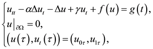(1.1)

where is a real-valued function on Let we make the following assumptions on functions

(1.2)

(1.3)

(1.4)

where are positive constants. And we assume that the external force belongs to the space and satisfies

(1.5)

for some given (possibly large) constant.

Wave equations, describing a great variety of wave phenomena, occur in the extensive applications of mathe- matical physics. Equation (1.1) can be regarded as a perturbed equation of a continuous Josephson junction where, see [1] . There is a large literature on the asymptotic behavior of solutions for strongly damped wave equations (see, for instance, [1] - [9] ). In [9] , the author showed the uniform boundedness of the global attractor for large strongly damping and obtained an estimate of the upper bound of the Hausdorff dimen- sion of an attractor for strongly damped wave Equation (1.1) when is independent of. But when the equations depend explicitly on, the case can be complex.

Recently, motivated by [6] , the authors have given a new explicit algorithm allowing to construct the expo- nential attractor, and this method makes it possible to consider more general processes in applications [10] [11] .

An exponential attractor is a compact semi-invariant set of the phase space whose fractal dimension is finite and which attracts exponentially the images of the bounded subsets of the phase space. In non-autono- mous dynamical systems, instead of a semigroup, we have a so-called (dynamical) process depending on two parameters (or for discrete times). The asymptotic behavior of non-autonomous dy- namical systems is essentially less understood and, to the best of our knowledge, the finite-dimensionality of the limit dynamics was established only for some special (e.g. quasiperiodic) dependence of the external forces on time. Indeed, there exists, at the present time, one of the different approaches for extending the concept of a glo- bal attractor to the non-autonomous case which is based on the embedding of the non-autonomous dynamical system into a larger autonomous one by using the skew-product flow. This approach naturally leads to the so- called uniform attractor which remains time-independent in spite of the fact that the dynamical system now depends explicitly on the time, see [12] . We note that however the uniform attractor reduces to an autono- mous system via the skew-product flow. It seems natural to generalize the concept of an exponential attractor to the non-autonomous case, see [11] [13] [14] . But in all these articles, the uniform attractor’s approach was used in order to construct an exponential attractor for the non-autonomous system considered and, consequently, an (uniform) exponential attractor remained time-independent. Since, under this approach, an exponential attractor should contain the uniform attractor, all the drawbacks of uniform attractors (artificial infinite-dimensionality and high dynamical complexity) described above are preserved for exponential attractors.

In the present article, we study exponential attractors of the system (1.1) based on the concept of a non-au- tonomous (pullback) attractor. Thus, in the approach, an exponential attractor is also time-dependent. To be more precise, a family of compact semi-invariant (i.e.,) sets of the dynami- cal process (1.1) is an (non-autonomous) exponential attractor if

1) The fractal dimension of all the sets is finite and uniformly bounded with respect to

2) There exist a positive constant and a monotonic function such that, for every and every bounded subset of,

(1.6)

We emphasize that the convergence in (1.6) is uniform with respect to and, consequently, under this approach, we indeed overcome the main drawback of global attractors [13] .

This article is organized as follows. In Section 2, we first provide some basic settings and show the absorbing and continuous properties in proper function space about Equation (1.1). In Section 3 and Section 4, we prove the existence of the uniform attractor and exponential attractor of Equation (1.1), respectively. Finally, we prove the existence of infinite-dimensional exponential attractor, and compare it with the non-autonomous exponential attractor in Section 5.

2. Preliminaries

We will use the following notations as that in Pata and Squassina [15] . Let be the (strictly) positive operator on defined by

with domain

and consider the family of Hilbert spaces with the standard inner products and norms, respec- tively,

and

Then we have

and the compact, dense injections

In particular, naming the first eigenvalue of, we get the inequlities

We recall the continuous embedding

and the interpolation results: given for any, there exists such that

and let

Equation (1.1) is equivalent to the following initial value problem in the Hilbert space E

(2.1)

where and

It is well known (see, e.g., [3] , [9] ) that, under the above assumptions, Equation (2.1) possesses, for every and a unique (mild) solution Thus, Equation (1.1) defines a dynamical process in the phase space by

(2.2)

Define a new weighted inner product and norm in as

for any

where is chosen as

(2.3)

Obviously, the norm in (2.3) is equivalent to the usual norm in.

Let

where is chosen as

(2.4)

and then the system (1.1) can be written as

(2.5)

where

Lemma 2.1 For any we have

where

(2.6)

Proof. Since is dense in, and; we only need to prove lemma 2.1 for any

By (2.4) and (2.6), elementary computation shows

The proof is completed. ,

Lemma 2.2 Let assumptions (1.2)-(1.5) be satisfied. For any initial data, there exists a positive con- stant depending only on the coefficients of (1.3) and (2.4) and such that the following dissipative esti- mate holds:

where is a monotonic function and where the positive number depends also on (but is indepen- dent of the concrete choice of).

Proof. Write Let be the solution of the system (2.5) with the initial

value Taking the inner product of (2.5) with, we have

(2.7)

By (1.2), (1.3) and Poincaré inequality, there exist two positive constants such that

(2.8)

(2.9)

By (2.4) and (2.6), Let By (2.8)-(2.9), we have

(2.10)

where By (2.7) and (2.10),

By Gronwall’s inequality, we have an absorbing property:

This completes the proof. ,

Theorem 2.1 Given any and for the solutions of (2.5) with any two initial data such that, we have the following Lipschitz continuity in E

for some.

The proof is similar to Theorem 2 in [15] . ,

Theorem 2.2 For the solutions of (2.5) with different external forces and satisfying (1.5) and with the initial data and, the following contiuity holds:

where and are independent of and

The proof is similar to Lemma 4 in [5] .

3. Existence of the Uniform Attractor

The dissipativity property obtained in Lemma 2.2 yields the existence of an absorbing set for the process on. In the following section, we assume that holds, where is specified in (3.11).

Theorem 3.1 The process possesses a uniform attractor in

Proof. We consider such that

(3.1)

and we introduce the splitting where satisfies

(3.2)

satisfies

(3.3)

and is the solution of

(3.4)

We now define the families of maps and in where

First step: We prove that is bounded in that the solution of (2.5) is starting in bounded sets of initial data. The system (3.2) can be written as

(3.5)

where,

(3.6)

Similar to Lemma 2.1, we have

where is as (2.6). Multiply (3.5) by, so we get

(3.7)

Similar to Lemma 2.2, applying (3.7) and Young, Poincaré, Gronwall inequalities, we obtain

Now we multiply (3.5) by and integrate over to obtain

(3.8)

with

Then from (3.8) we have

i.e.,

(3.9)

for the first term on the right-hand side of (3.9), we have

(3.10)

By (3.9), (3.10), and Lemma 2.2, there is such that for all

(3.11)

let using the Gronwall’s lemma, we have

(3.12)

By (1.2), (1.3) and (2.8), (2.9), from (3.12), we obtain

(3.13)

Lemma 2.2 and (3.13) imply that is bounded in.

Second step: Let, we will prove that there exists independence of such that

Multiply (3.3) by, we thus obtain

due to Gronwall and Poincaré inequalities, then

(3.14)

Since the embedding is compact, (3.13), (3.14) and the following lemma imply that is compact in.

Lemma 3.1 (see [16] ) Let be a complete metric space and be a subset in, such that

with and is compact in, then is compact in.

Third step: Let, the same arguments in the Equation (3.4) lead to

(3.15)

Then from (3.15), Lemma 2.2, and the compactness of, the system (2.5) exists a uniform attractor in

It is easy to see that the process

defined by (2.5) has the following relation with:

(3.16)

where is an isomorphism of

Since the process possesses a uniform attractor by (3.16), also possesses a uniform attractor ,

4. Existence of Exponential Attractors

The main result of this section is the following theorem.

Theorem 4.1 Let the function f and the external force g satisfy the above assumptions. Then, for every ex- ternal force g enjoying (1.5), there exists an exponential attractor of the dynamical process (1.1) which satisfies the following properties:

1) The sets are semi-invariant with respect to and translation-invariant with respect to time-shifts:

(4.1)

where and is the group of temporal shifts,

2) They satisfy a uniform exponential attraction property as follows: there exist a positive constant and a monotonic function (both depending only on) such that, for every bounded subset of, we have

(4.2)

3) The sets are compact finite-dimensional subsets of

(4.3)

where the constant is independent of and.

4) The map is Hölder continuous in the following sense:

(4.4)

where the positive constants and are independent of and, denotes the symme- tric Hausdorff distance. In particular, the function is uniformly Hölder continuous in the Hausdorff metric:

(4.5)

where and are also independent of and.

Proof. Firstly, we construct a family of exponential attractors for the discrete dynamical processes associated with Equation (2.5). According to Lemma 2.2, it only remains to construct the required exponential attractors for initial data belonging to the ball

where is a sufficiently large number depending only on given in (1.5), is a uniform absorbing set for all the processes generated by Equation (1.1). Moreover, from Theorem 2.1, Theorem 2.2 and Theo- rem 3.1, it follows Lipschitz continuity and smooth properties for the difference of two solutions and. Thus, by Theorem 2.1 in [13] , the family of discrete dynamical processes possess exponential attractors For obtain- ing exponential attractors of the family of dynamical processes, we need the Hölder continuity of the processes with respect to the time, see the following lemma.

Lemma 4.1 Let the above assumptions on Equation (1.1) hold. Then, for every we have

(4.6)

where the constant depends on, and is independent of Moreover, for every we also have

(4.7)

where is a positive number and the positive constant depends on but is independent of and.

Proof. Note that there is a such that

and is uniformly bounded in and Lemma 2.2, which imply the Hölder continuity (4.6). In order to verify (4.7), we note that, due to (4.6) and Theorem 2.2, for every, we have

where all the constants depend on, but are independent of and Using the previously mentioned interpolation inequality in Section 2 finishes the proofs of estimate (4.7). ,

Now, we can define the exponential attractors for continuous time by the following formula

with respect to The proofs of the semi-invariance with respect to and translation-invariance with respect to time-shifts is similar to [11] [13] . Estimate (4.2) follows in a standard way from Lemma 2.2, Theorem 3.1 for the processes. Thus, it only remains to verify the finiteness of the fractal dimension of. In order to prove this, we first note that, according to the Hölder continuities Theorem 2.1 in [13] and (4.7), we have

for all, and. Since the map are uniformly Lipschitz conti- nuous, Theorem 3.1 in [13] implies that

for a given, and some constant and which are independent of. The proof of Theorem 4.1 is completed. ,

5. Infinite-Dimensional (Uniform) Exponential Attractor and Non-Autonomous Exponential Attractor

Finally, we compare the non-autonomous exponential attractor obtained above with the so-called infinite-dimensional (uniform) exponential attractor constructed in [11] [13] . To the existence of the uniform at- tractor for strongly damped wave equations, we use the results in [4] and [5] as a model example.

Let be some external force. Let be the hull of in, i.e.,

where denotes the closure in. Evidently, for any.

Using the standard skew product flow in [4] and [5] , for every external forces satisfying (1.5), we can embed the dynamical process into the autonomous dynamical system acting on the extended phase space via

It is known that is a semigroup. If this semigroup possesses the global attractor, then, its projection onto the first component of the Cartesian product is called the uniform at- tractor associated with problem (1.1).

It is also known that the uniform attractor exists under the relatively weak assumption that the hull is compact in, but, unfortunately, for more or less general external forces its Haus- dorff and fractal dimensions are infinite. Instead, the following estimate for its Kolmogorov’s -entropy holds, see [4] .

Proposition 5.1 Let the above assumptions hold and the hull of the initial external forces be compact. Then, Equation (1.1) possesses the uniform attractor and its -entropy can be estimated in terms of the -entropy of the hull as follows:

(5.1)

for some positive constants and depending on.

Definition 5.1 [11] [13] A set is an (uniform) exponential attractor of Equation (1.1) if the fol- lowing properties are satisfied:

1) Entropy estimate: is a compact subset of the phase space which satisfies estimate (5.1) (possibly, for larger constants and).

2) Semi-invariance: for every there exists such that for all

3) Uniform exponential attraction property: there exists a positive constant and a monotonic function such that, for every and every bounded subset, we have

(5.2)

[13] points out that a uniform exponential attractor can be constructed if the (non-autonomous) exponential attractor has been constructed, so we have

Theorem 5.1 Let the assumptions of Theorem 4.1 hold and let, in addition, the hull of some external forces satisfying (1.5) be compact. Then, there exists a uniform exponential attractor for problem (1.1) which can be constructed as follows:

Remark 1 When, Equation (1.1) reduces to the following damped wave equation on a bounded domain with smooth boundary:

(5.3)

Equation (1.1) reduces to the damped wave equation modeling the Josephson junction in superconduction which was studied by many authors (see [1] [6] [17] ). We assume that the function satisfy (1.2)-(1.4). The Equation (5.3) also possesses a finite dimensional exponential attractor.

Remark 2 When, Theorem 4.1 remains valid for the following strongly damped wave equation was studied by many authors (cf. [7] [18] ):

if we assume that the function satisfy (1.2)-(1.4).

Acknowledgements

This work is supported by the National Natural Science Foundation of China (11101265) and Shanghai Edu- cation Research and Innovation Key Project of China (14ZZ157).

Conflicts of Interest

The authors declare no conflicts of interest.

References

[1]	Landahl, P.S., Soerensen, O.H. and Christiansen, P.L. (1982) Soliton Excitations in Josephson Tunnel Junctions. Physical Review B, 25, 5337-5348.
[2]	Dell’Oro, F. and Pata, V. (2012) Strongly Damped Wave Equations with Critical Nonlinearities. Nonlinear Analytical TMA, 75, 5723-5735. http://dx.doi.org/10.1137/0522057
[3]	Ghidaglia, J.M. and Marzocchi, A. (1991) Longtime Behavior of Strongly Damped Nonlinear Wave Equations, Global Attractors and Their Dimension. SIAM Journal on Mathematical Analysis, 22, 879-895. http://dx.doi.org/10.1137/0522057
[4]	Li, H. and Zhou, S. (2012) Kolmogorov ε-Entropy of Attractor for a Non-Autonomous Strongly Damped Wave Equation. Communications in Nonlinear Science and Numerical Simulation, 17, 3579-3586. http://dx.doi.org/10.1016/j.cnsns.2012.01.025
[5]	Li, H. and Zhou, S. (2008) On Non-Autonomous Strongly Damped Wave Equations with a Uniform Attractor and Some Averaging. Journal of Mathematical Analysis and Applications, 341, 791-802. http://dx.doi.org/10.1016/j.jmaa.2007.10.051
[6]	Prizzi, M. (2009) Regularity of Invariant Sets in Semilinear Damped Wave Equations. Journal of Differential Equations, 247, 3315-3337. http://dx.doi.org/10.1016/j.jde.2009.08.011
[7]	Sun, C. (2010) Asymptotic Regularity for Some Dissipative Equations. Journal of Differential Equations, 248, 342-362. http://dx.doi.org/10.1016/j.jde.2009.08.007
[8]	Yang, M. and Sun, C. (2009) Dynamics of Strongly Damped Wave Equations in Locally Uniform Spaces: Attractors and Asymptotic Regularity. Transactions of the American Mathematical Society, 361, 1069-1101. http://dx.doi.org/10.1090/S0002-9947-08-04680-1
[9]	Zhou, S. (1999) Global Attractor for Strongly Damped Nonlinear Wave Equations. Functional Difference Equations, 6, 451-470.
[10]	Eden, A., Foias, C., Nicolaenko, B. and Temam, R. (1994) Exponential Attractors for Dissipative Evolution Equations. Research in Applied Mathematics, 37, John-Wiley, New York.
[11]	Efendiev, M., Miranville, A. and Zelik, S. (2003) Infinite Dimensional Attractors for a Non-Autonomous Reaction-Diffusion System. Mathematische Nachrichten, 248-249, 72-96. http://dx.doi.org/10.1002/mana.200310004
[12]	Chepyzhov, V.V. and Vishik, M.I. (2002) Attractors for Equations of Mathematical Physics. AMS College Publication, Providence.
[13]	Efendiev, M., Zelik, S. and Miranville, A. (2005) Exponential Attractors and Finite-Dimensional Reduction for Nonautonomous Dynamical Systems. Proceedings of the Royal Society of Edinburg Sectection A, 135, 703-730.
[14]	Miranville, A. (1998) Exponential Attractors for Non-Autonomous Evolution Equations. Applied Mathematical Letters, 11, 19-22. http://dx.doi.org/10.1016/S0893-9659(98)00004-4
[15]	Pata, V. and Squassina, M. (2005) On the Strongly Damped Wave Equation. Communications in Mathematical Physics, 253, 511-533. http://dx.doi.org/10.1007/s00220-004-1233-1
[16]	Atlas, A. (2005) Regularity of the Attractor for Symmetric Regularized Wave Equation. Communications on Pure and Applied Analysis (CPAA), 4, 695-704. http://dx.doi.org/10.3934/cpaa.2005.4.695
[17]	Ogawa, T. and Takeda, H. (2011) Large Time Behavior of Solutions for a System of Nonlinear Damped Wave Equations. Journal of Differential Equations, 251, 3090-3113. http://dx.doi.org/10.1016/j.jde.2011.07.034
[18]	Pata, V. and Zelik, S. (2006) Smooth Attractors for Strongly Damped Wave Equations. Nonlinearity, 19, 1495-1506. http://dx.doi.org/10.1088/0951-7715/19/7/001