Analyses of Physical Data to Evaluate the Potential to Identify Class I Injection Well Fluid Migration Risk ()
1. Introduction
The United States Environmental Protection Agency (USEPA) is tasked with protecting underground sources of drinking water as a part of the Safe Drinking Water Act (SDWA). USEPA’s permitting authority to govern underground injection programs results from the Underground Injection Control (UIC) Program, promulgated in 1981 pursuant to the Safe Drinking Water Act (SDWA) under 40 CFR 144 and 146. The Federal regulations include an extensive set of definitions concerning the types and purposes of injection wells. These regulations were aimed at regulating disposal of waste via underground injection, and are clearly focused on the injection of any other liquid that might impact groundwater quality, particularly hazardous materials. For example, the Federal regulations segregate the wells into the following classes (summarized from 40 CFR 146) [1] [2] :
1) Class I injection wells are identified as either wells used by generators of hazardous waste or owners and operators of hazardous waste management facilities which inject those hazardous waste beneath the surface. The requirement is that the waste be injected beneath the lower-most formation of an underground drinking water source and more than ¼ mile horizontally from it. This requirement includes other industrial and municipal disposal wells which inject fluids beneath the lower-most formation containing potable drinking water supplies. Municipal wastes, which are not specifically defined in federal regulations, are wastes associated with sewage effluent that has received treatment. With the exception of desalination wastes, disposal of municipal waste through injection wells is currently practiced only in Florida. In Florida, this waste disposal practice is often chosen due to a shortage of available land, strict surface water discharge limitations, extremely permeable injection zones, and cost effectiveness. Currently, there are 473 Class I wells in the United States, of which 123 are hazardous, and 350 are non-hazardous or municipal wells. Texas has the greatest number of Class I hazardous wells (64), followed by Louisiana (17). Florida has the greatest number of nonhazardous wells (all but 2 of which are injection wells used for disposal of treated municipal wastewater), followed by Texas and Kansas [3] .
2) Class II wells are used to inject fluids that are brought to the surface in connection with conventional oil and natural gas production, or the enhancement of recovery of oil and natural gas and the storage of hydrocarbons (usually handled by the Department of Interior as opposed to USEPA). There are 168,000 Class II wells [4] .
3) Class III wells are utilized for the extraction of minerals. There are 22,000 Class III wells [4] .
4) Class IV wells are used by generators of hazardous radioactive waste which inject water below the lower-most drinking water zone. None has application in the injection processes described herein, but their existence may inhibit such efforts. GWPC (2007) reports 33 Class IV wells [4] .
5) Class V wells are all wells that are not included in Class I, II, III, IV or VI. The wells described herein for underground injection programs generally described as aquifer storage and recovery, saltwater intrusion barrier, or managed aquifer recharge are all Class V wells. 460,000 wells exist in the US [4] .
6) Class VI wells are used to dispose of the greenhouse gas carbon dioxide; a by-product of fossil fuel use, cement processing and other industrial processes. No Class VI wells have yet been permitted.
Much of regulatory environment relates to the type of well proposed and its use. The classes are generally based on the kind of fluid injected and the depth of the fluid injection compared with the depth of the lowermost USDW. Figure 1 illustrates the well type for a figure derived from EPA Region 9.
Under the rules were established under the authority of Safe Drinking Water Act approved in 1974 and amended in 1986 and 1996, states can apply to take on oversight and enforcement the underground injection control (UIC) program by adopting regulations at least as stringent as federal rules, have primacy under Section 1413. Federal rules for these state UIC rules are provided in parts 145 and 147 [5] [6] . Over 40 states have delegation.
The regulations set forth types of materials that are permitted for use in well construction and minimum design criteria and testing to insure well integrity. Wastes are an unavoidable by-product of a myriad of manufacturing processes which create thousands of waste products used in the course of everyday living. GWPC notes that “Since the passage of several legislative acts in the 1970’s regulating waste disposal into water, air, and landfills, underground injection has grown in importance [7] ”. In the petroleum industry alone, about 900 billion gallons of wastewater are generated each year in the United States from nearly a million oil & gas wells. If disposed of at the surface, this water would pose a risk of contaminating surface waters or groundwater used for drinking purposes. Consequently, these wastes are pumped underground through wells constructed specifically for those injecting waste products.
In addition to the oil and gas industry, millions of gallons of product waste is generated in the steel, plastics, pharmaceuticals, and many others industries. All of these wastes have varying degrees of hazard. To assess the hazard, the chemical constituents of the wastes are required. Additionally, many millions of gallons of liquid wastes are generated in large municipalities from secondary treated wastewater. While the utility industry continues to research and implement ways to reduce waste by recycling and improving treatment processes, generated wastes still require disposal.

Figure 1. Example of Different Types of Wells Source: USEPA [8] .
2. Literature Review
The history of injection wells goes back to the 1900s in the United States, primarily with respect to oil and gas production and mining. In these cases, the injected water was used to flush the desired components to the surface. At the time, little consideration was given to the impacts of the injected fluids and how that may react with the native hydrogeologic conditions. With the advent of improved pumping systems and power, the number of injection wells increased substantially in the 1930s, when the first shallow industrial waste well was completed [9] . Deeper disposal of chemical wastes was initialed in the 1950s [9] , while injection wells continued to be used for oil and gas production. Most of the early injection wells were oil production wells converted for wastewater disposal. In the 1950s, injection of hazardous chemical and steel industry wastes began. At that time, four Class I wells were reported; by 1963, there were approximately 30 injection wells. In the mid 1960s and 1970s, Class I injection began to increase sharply, growing at a rate of more than 20 wells per year [3] . Class I injection wells are identified as wells used by generators of hazardous waste or owners and operators of hazardous waste management facilities to inject those hazardous waste beneath the surface. The requirement is that the waste be injected beneath the lower most formation within 1/4 mile of a well bore for an underground drinking water source. Other industrial and municipal disposal wells which inject fluids beneath the lower most formation containing potable drinking water supplies are also included. Injection wells were believed to be superior to other disposal practices for hazardous waste materials to maximize the separation of wastes from human contact. The practice was supported by industry and regulatory agencies as long as not adverse impacts were noted.
The increased use of injection wells raised public concerns about environmental and aquifer protection. For example, corrosion caused migration of wastes to the surface in April 1968 at Hammermill Paper Company’s No. 1 well in Erie, PA. The well ruptured, spilling pulping liquor onto the land and into Lake Erie. In Beaumont, TX, a ruptured casing caused contamination in an aquifer above the injection horizon at Velsicol Chemical Company [3] . Concerns about earthquakes in the Denver area creating a pathways for leakage from the Rocky Mountain Arsenal well operating from 1961-1966 [10] [11] . The potential for contamination of drinking water supplies from upward migration of wastes from thousands of wells, with little notice to water users, creates a significant potential for adverse public health impacts.
Rish et al. and USEPA deemed the probability of containment migration ranging from one-in-a-million to onein-a-quadrillion [3] [12] . The low risk is attributed to the use of multiple barriers to migration created by engineered systems and geologic knowledge. However there are wells that leak or are suspected of leaking in most states with Class I, II, III or IV wells.
The focus here is the Class I municipal injection wells, which is primarily a Florida issue. Class I wells in Florida were selected because there are over 200 of them and they are installed similarly. The injection fluids are virtually identical as well, so numerous variables with respect to chemical risk are eliminated.
The recorded instance of deep well injection in Florida was in 1943. Brine produced as a by-product of oil extraction from the Sunniland oil field in Collier County was disposed of by pumping it back into the lower zones of the Floridan aquifer [13] [14] . The first injection of municipal effluent into brackish zones of the Upper Floridan Aquifer System began with a single injection well in Broward County just west of Lighthouse Point in 1959 [14] . Due to unique hydrologic conditions, from 1959 to 1970, the volume of municipal and industrial liquid wastes injected into the Floridan Aquifer System increased gradually from 98 to 465.6 million gallons per year [14] . Permitting was handled on a case-by-case basis using unspecific federal and state rules to maximize the protection of the overlying aquifers [15] .
Expansion of the injection well program in the state was limited until the 1970s when the Clean Water Act was approved by Congress. Both alternatives are less expensive due to the less stringent treatment requirements relative to canal discharges. Injection of treated municipal wastewater into the saltwater-filled Boulder Zone began in 1971 at a wastewater treatment plant in Miami-Dade County [14] [16] . The decade of the 1970’s domestic injection wells were developed along the east coast of Florida, from Dade County to Brevard County, and on the west coast in Pinellas County. Also during the same period, several industrial injection wells were developed in the Florida panhandle, and in Polk, Indian River, and Palm Beach Counties [15] . After Florida’s UIC program was approved to receive primacy via delegation, there was a rapid increase in total volume of injected wastewater and the number of deep injection wells [17] . In the early 1980’s, the USEPA found that some municipal deep injection wells in the Tampa Bay and central Florida areas may have caused fluid movement above the injection zone [15] . Where there appeared to be vertical movement of the injected fluid into the lower monitoring zone, the well was deemed to be “leaking”. The determination of leakage was made through elevated concentrations of ammonia and Total Kjeldahl Nitrogen (TKN), and depressed salinity, relative to native water in the Floridan Aquifer reported in monitoring wells in zones overlying the injection zone [18] . As of 2007, 210 Class I injection wells are used to dispose of over 500 MGD of secondary treated wastewater in the State, making Florida the state with the largest UIC program for wastewater disposal. It should be noted that all wastewater injection meets secondary treatment requirements, directed principally toward the removal of bio-degradable organics and suspended solids. Elevated concentrations of ammonia and total kjeldahl nitrogen, and depressed salinity relative to native water in the Floridan aquifer, were reported in monitoring wells in zones overlying the injection zone in Miami-Dade County [19] .
Both FWEA and USEPA conducted risk studies to evaluate the relative risk assessment program to compare ocean outfalls, deep wells and surface water discharges [3] [19] . The intention of both assessments was to provide a comparative risk of each practice. Water quality data, relative to disposal of wastewater treatment plant effluent were gathered, along with water quality data on the receiving waters, from utilities [18] . The results indicated that health risks associated with deep wells were generally lower than those of the other two alternatives [18] . The proximity of injection wells to aquifer storage and recovery wells was a determining factor relative to injection well risk [18] .
However, in neither case was there enough information to perform and actual modeling of an injection well due to a lack of data about the geophysical properties of individual wells, and a lack of models that could resolve the density differential and dilution issues. What was left unaddressed by either study, or subsequent rule-making, was a means to understand or predict methods and/or correlation of factors that lead to fluid migration and subsequent failure (i.e., leaks in casing that result in migration into USDW), which is purpose of this investigation.
The goal of this paper is to evaluate whether there is a mechanism to determine which wells are most likely to have leakage potential. The investigation was because Florida is the only state that uses Class I wells for treated effluent. Most states have older wells, and more difficult waste issues. As a result, the potential risks in all other UIC states will likely exceed those in Florida. The Florida case study provides a pathway to investigate UIC program in the other states, many of which have larger UIC programs than Florida. Texas, for example has over 4 times the number of wells as Florida, and most are industrial waste sites, as opposed to treated effluent.
3. Methodology
3.1. Data Collection
The project comprised two phases, data collection and data analysis. The data was collected from participating utilities and regulatory agencies. Data was collected from each of the regulatory District Offices that regulated injection wells: Central, Southeast, South, and Southwest. As a part of the process, a hard copy of the UIC permit for every Class I Well issued by FDEP was obtained. In addition, the files were scanned to collect construction and stratigraphy data from all the well completion reports. All permit files were scanned and are available in FAU files. The next step was to develop a database of physical and permit parameters for all the Class I injection wells in the state.
Variables of interest were first identified as they may provide the reasoning for regional differences and frequent occurrences of upward migration in certain regions. The identified parameters were carefully extracted from each of the well permit documents and systematically compiled in a tabular form. The table is sorted by FDEP map reference number. This set of collected data is a representation of the deep injection well inventory as of September, 2007. Descriptions of the collected data set are provided as follows:
• District: District in which the DIW resides
• County: County in which the DIW resides
• Usage: Classification of wells including hazardous or non-hazardous. Non-hazardous wells include municipal, reverse osmosis, combined, and industrial.
• Leaking Status: A leaking well indicates confirmed or possibly detected upward migration into or below the USDW base; it does not include leaking caused by any physical damage of the well itself.
• Operational Status: Operational status is either active, pending, abandoned, or converted.
• Number of DIW: The number of individual Class I Wells onsite to accommodate the designed injection capacity.
• DIW Depth: A measure of depth in feet of the deepest point of the DIW opening.
• DIW Final Casing Depth: A measure of depth in feet of the most interior and deepest well casing that is installed at the final construction stage.
• DIW Injection Horizon: A distance in feet measuring the difference between the well and its final casing depth.
• DIW Final Casing Diameter: A measure of diameter in inches of the most interior and deepest well casing that is installed at the final construction stage.
• DIW Peak Flow: A measure of injection capacity in million gallons per day at peak flow.
• Number of Monitoring Wells: The number of wells onsite for monitoring Class I wells.
• Depth of Lower Monitoring Zone: A depth measurement of the lower opening of the monitoring well in feet. If more than two monitoring zones present at any given site, the lowest monitoring zone is considered.
• Depth of Upper Monitoring Zone: A depth measurement of upper opening of the monitoring well in feet. If more than two monitoring zones present at any given site, the upper most monitoring zone is considered.
• Distance from Injection Zone to Lower Monitoring Well: A distance in feet measuring the difference between final casing depth and lower monitoring zone depth.
• Distance from Injection Zone to USDW: A distance in feet measuring the difference between final casing depth and the base of USDW zone.
• Clay Zone Boundary: Indicates whether a clay zone is present above the injection point. The clay zone boundary is categorized as solid, interspersed, or none.
• Clay Zone Thickness: A thickness measurement in feet of the clay zone above the injection point. Zero indicates an absence of the clay zone.
• Boulder Zone: Indicates whether the injection of the Class I Well is in boulder zone.
• Tubing and Packer: Indicates whether the Class I Well uses tubing and packer.
• Collecting the following variables was attempted. However, limited data was available from the UIC permit.
• Vertical and Horizontal Hydraulic Conductivity (K): The measure of waters ability to maneuver through a porous media. It is the rate of flow per unit time per unit cross-sectional area.
• Porosity: A measure of how densely materials are packed within a media. It is the ratio of pore volume to total volume.
It should be noted that not all of this information was available for all wells, especially the aquifer parameters of the older wells (porosity, hydraulic conductivity). For these missing data, some assumptions or categorization of wells was used based on adjacent findings.
3.2. Data Analysis
To better understand the differences between the regions, the collected data was managed, summarized, and analyzed with XLStat® Correlation analysis was used indicates whether the variable is related to other variables on an individual basis. The benefit of this analysis is to identify parameters that are obviously related. However this works best when there are a limited number of variables (as opposed to the 24 variables here).
The factor analysis (FA) method dates from Spearman [20] . There are two main types of factor analysis: Exploratory factor analysis (EFA) and Confirmatory factor analysis (CFA). XLStat® uses EFA to reveal the potential existence of underlying factors within data containing a very large number of measured variables. For EFA, the structure linking the variables is initially unknown, but the number of factors is assumed. CFA uses a method identical to EFA but the structure linking underlying factors to measured variables is assumed to be known.
Principle Component Analysis (PCA) is one of the most frequently used multivariate data analysis methods. Given a table of quantitative data (continuous or discrete) in which n observations (observations, products, etc.) are described by p variables (the descriptors, attributes, measurements, etc.), if the number of p variables is high, it is impossible to understand the structure of the data Instead, PCA permits:
• The visualization of the correlations between variables that will permit the number of variables to be reduced and correlated;
• The ability to obtain non-correlated factors which are linear combinations of the initial variables so as to use these factors in modeling methods such as linear regression, logistic regression or discriminant analysis.
The resulting PCA factors incorporate the initial variables into correlated groups to reduce the dimensionality of p multi-attributes to two or three dimensions. PCA is a special case of factor analysis (where n, the number of factors, equals p, the number of variables). While FA assumes a number of factors, PCA is used to reduce the number of variable to factor sets, while maximizing the unchanged variability in order to obtain independent (non-correlated) factors. The mathematics of PCA uses an orthogonal transformation convert observations of possibly correlated variables into a set of values of linearly uncorrelated variables called principal components. PCA uses a multivariate statistical parameter called an eigenvalue, which is a measure of the amount of variation explained by each principal component. PCA summarizes the variation in a correlated multi-attribute to a set of uncorrelated components, each of which is a particular linear combination of the original variables [21] . The intent was to see if factors that might contribute to a well no longer being used could be identified. With the PCA analysis, all factors in excess of 1 are kept. Those with factor values under 1.0 are assumed to contribute little to the overall explanation of the results. It is desirable that the factors represent at least 70 percent of the resulting eigenvalues. Once the factors are identified and eigenvalues are analyzed to determine which variable contribute most to the factor. The investigator should look for values that are greater than 0.6 or 0.7. A Scree Plot is a simple line segment plot that shows the fraction of total variance in the data as explained or represented by each component [22] .
Discriminant function analysis (DA) is also closely related to PCA in that they both look for linear combinations of variables to explain the data. Using these techniques, the factors affecting each component can be determined, allowing the investigator to evaluate common and differing results by the factors most affecting the results. A biplot display of both factors and factor loadings is an effective way of studying the relationships between variables, and the interrelationship between observations and the variables [23] . The methodology used to derive the DA coefficients parallels one-way MANOVA, except that DA searches for linear combinations of the quantitative variables that provide maximal separation between the classes or groups. The idea is to be able to graphically separate the options into distinct groups. The correlations among the multivariate attributes used in the DA analysis are revealed by the angles between any two DA loading vectors. For each variable, a DA load vector is created by connecting the X-Y origin and the multiplied value of F1 and F2 loadings in the biplot [21] . The angles between any two variable vectors will be:
1) Narrower (<45˚) if the correlations between these two attributes are positive and larger 2) Wider (around 90˚) if the correlation is not significant 3) Closer to 180˚ (>135˚) if the correlations between these two attributes are negative and stronger The membership of each factor in question can be grouped using Mahalanobis distances. In general, the Mahalanobis distance is a measure of distance between two points in the space defined by two or more correlated variables taking account of the covariance structure [21] . Using Mahalanobis distances for each variable, the location of the point that represents the means for variables in the multivariate space defined by the variables in the model can be determined. These points are called group centroids [24] . For each case, the Mahalanobis distances from each of the group centroids can be computed. Since the probability that a case belongs to a particular group is proportional to the Mahalanobis distance from the group’s centroid, each case is classified as belonging to the group to which it is closest, that is, where the Mahalanobis distance is smallest [21] .
4. Results and Discussion
From an evaluation of the data the following facts were gleaned:
1) 65 percent of sites have only one well, while 25% have two. One site in Miami Dade County has 17, while another has 8. This suggest that that majority of the wells have a low capacity or they are used for back-up disposal only, requiring fewer wells for disposing treated wastewater.
2) The current cost of a deep injection well is between $5 and 6 million.
3) As of September 2007, there was a total of 129 Class I well sites and 216 wells in Florida [4] .
4) The operational status of the wells includes 22 pending, 20 non-active, and 174 active. Among the 174 active wells, only 1 was classified as a hazardous well and the rest (173) were non-hazardous wells. The only active hazardous well resides in Polk County, which has been carefully monitored to ensure its performance.
5) The permitting process is constantly evolving to add more wells. Only two sites are abandoned (both in Miami-Dade County) and 85 sites have been active for over 5 years. Pinellas County converted a series of its wells to Class V ASR wells.
6) The number of wells and well sites has increase each decade since 1960. The first well, now abandoned was constructed in 1943;
7) Of the four FDEP districts involved, the southeast District has 48% of the well sites, followed by south District (southwest Florida), Southwest (Tampa Bay) and Central. The Southeast District encompasses the three most populous counties in Florida: Miami-Dade, Broward, and Palm Beach, so it is no surprise the greatest number of wells is in southeast Florida. The Southeast District is also where the Boulder zone was first discovered and has been studied extensively. In southeast Florida, the Boulder zone is viewed as an ideal site for accepting large amount of injected fluid.
8) 62 percent of the sites have tubing and packer wells. Tubing and packer wells are primarily used for concentrate disposal 9) Half the wells, primarily in South and Southeast Florida, exceed 3000 feet deep, with a final casing set at over 2500 feet deep.
10)Nearly half the wells were 24 inches in diameter and can inject 15 MGD. 25% pf the wells are less than 16 inches in diameter and are permitted to pump under 8 MGD.
11)The injection horizon exceeds 500 feet in two thirds of the well sites, and over 75 percent of the wells.
12)Monitoring wells are required to be permitted and constructed to collect data in two monitoring zones at a distance of less than 150 feet from the injection wells. 57% of sites have only one monitoring well. 20% have two. 8.8% have over 5. Since there is only one monitoring well on site, the majority of the monitoring wells are either dualor multi-zone.
13)Virtually all the wells have steel casings. Only two sites have fiberglass and none have PVC due to the depth.
14)Half the well sites have a significant clay later (generally over 300 feet) between the injection zone and the surficial aquifer. Virtually all of these are in south and southeast Florida. 13 sites have no significant clay layer, which are primarily in the Tampa Bay area.
Lower zone monitoring wells are designed to monitor the aquifer zone immediately above the injection horizon. They are also required to be below the base of the USDW. Figure 2(a) illustrates that 64 percent of lower monitoring wells have depths ranging from −2000 feet to –1000 feet. In comparison the upper monitoring zone wells are required to be within or above the USDW. Figure 2(b) shows the depths between of the UMZ. The deepest wells are −2000 feet and −1500 feet deep (20%), while 34 percent at depths range from −1500 feet to −1000 feet, 27.5% −500 to −1000 and the rest less than 500 feet. These values are 500 feet or more above the lower monitoring zone wells.
Table 1 shows the wells by district. Figure 3 and Figure 4 show the Southeast District has the deepest set of the monitoring wells, followed by the South, Central, and Southwest Districts. Monitoring wells usually reside below and within the USDW base. The graphs demonstrate the USDW varies throughout the state, and the depths correspond to hydrogeological formations.
Figure 5 and Figure 6 provide well depths and final casing depths, respectively. Both interval plots show an identical descending order from the deepest to the shallowest: Southwest, Central, South, and Southeast. In looking at the final casing depth and the final well depth, there is no clear correlation between the injection ho-
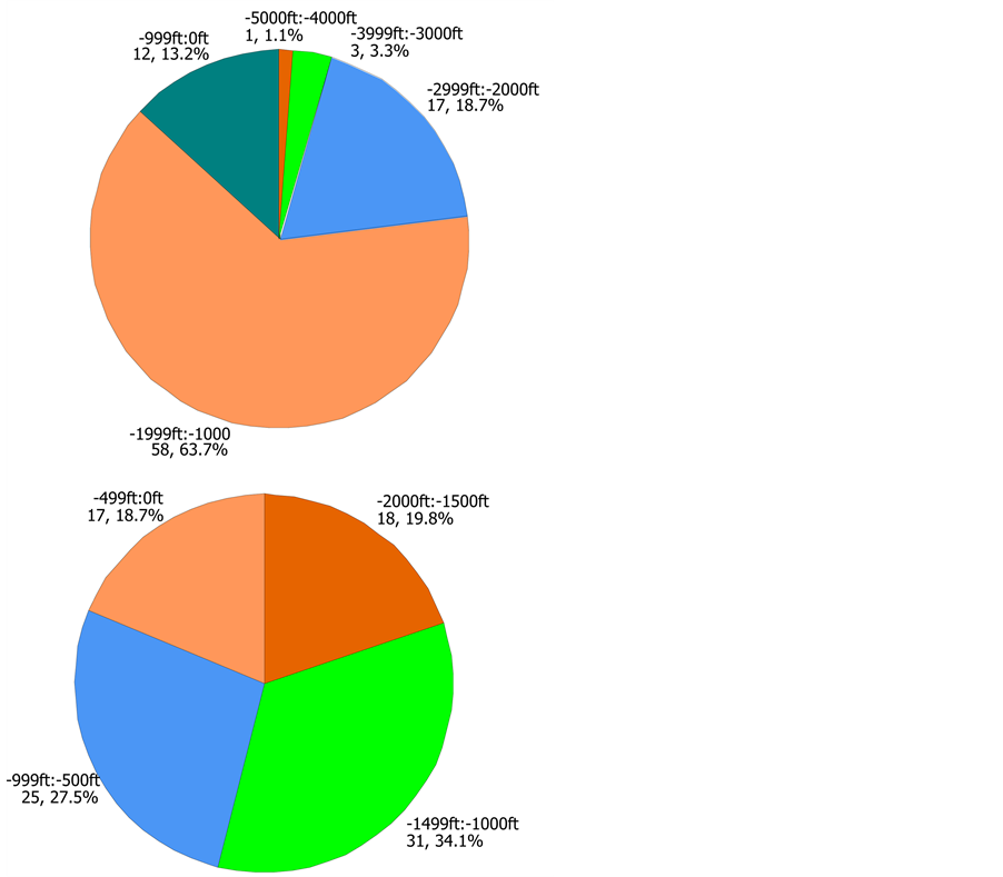
Figure 2. Depth of lower and upper monitoring zone wells.

Table 1. Class I well program in Florida.
rizon(s) and the depths, but the Central Florida (Central and Southwest Districts) have a wider injection horizon compared to South Florida (Southeast and South Districts) and both are generally shallower. In the case of southwest Florida (Tampa Bay), much shallower.
The number of sites that are suspected of fluid migration is 21. The number of wells with fluid migration is

Figure 3. Depth of lower monitoring well by district interval plot.

Figure 4. Depth of upper monitoring well by district interval plot.
highest in the Tampa Bay area (most converted to ASR wells as a result of consent decrees). Figure 7 shows the percent of wells leaking in each district. Figure 8 shows the operational status of DIWs that are or are suspected of leaking within each district. The Central District has the least number of wells; however, it has the most leaking well sites: 40 percent of its total well sites, followed by 36 percent for the Southwest District and 20 percent for the Southeast District. No wells with fluid migration have been documented in the South District. Even though the Central has 40 percent of its well sites that have detected upward migration, all the wells are still in operation because treatment levels have been upgraded to meet reuse requirements, including high level disinfection. Two well sites (both in SE Florida) had construction issues noted at the sites that are suggested as the cause of the apparent leaks. What is known is that two different contractors were used on these sites. A third contractor has successfully drilled 83/83 wells in south Florida, which suggested that the driller may play a major role in migration issues. Unfortunately data on the drillers was not available in the FDEP files.
Distance from final casing and the base of USDW represents the vertical distance between the injection and USDW zones. The separation isolates the USDW from contamination by the injected fluid. Figure 9 shows the wells with fluid migration have a mean value of 2561 feet of vertical depth compared to 3001 feet for the remaining wells. The comparison depicts a safer practice for keeping the two zones further apart by deepening the injection wells. In these figures, Y means fluid migration, and N means no fluid migration detected.
Next, correlation analysis was developed for all variables against one another. The concept was to use PROC CORR in SAS to identify those variables with significant correlation (>0.0001). Eighteen sets of variables met this definition:
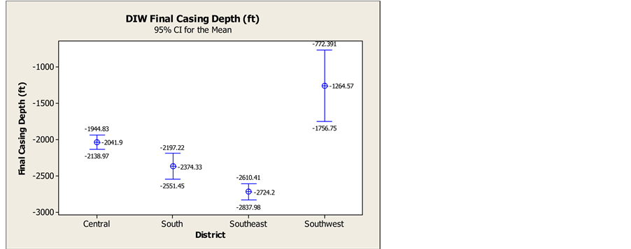
Figure 6. DIW final casing depth by district.

Figure 7. DIW leaking status by district.

Figure 8. Status of leaking wells by district.
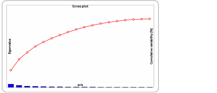
Figure 9. Scree l = plot of eignevalues.
• Install date and fluid migration
• Upper monitoring zone (UMZ)and lower monitoring zone (LMZ) depth
• Casing depth and confining unit
• Casing depth and UMZ
• Casing depth and LMZ
• Total depth of well and-distance between injection zone and LMZ
• Total depth of well and confining unit
• UMZ and casing depth
• Casing depth and LMZ
• Casing depth and depth of well None of these are a surprise, although the install day/fluid migration pairing is interesting.
With 19 variables and 91 sites to evaluate to determine if there is any indicator of potential leakage, reducing the number of factors is needed. Using these variables, principal component analyses (PCA) was performed. All variables were inserted in the PCA with the dependent variable being leakage. Table 2 shows the eigenvectors for the variable set, with a Scree plot is shown in Figure 9. Eigenvectors were developed with the assumption of 6 factors (all > 1) being retained. Each of the eigenvectors was evaluated to determine the major inputs to each.
The factors were generally defined as follows:
Table 2. Eigenvalues (retain Factors > 1.0).
• Factor 1—the well construction depth
• Factor 2—an inverse relationship to flow volume at the site
• Factor 3—install date
• Factor 4—the use of tubing and packers (higher percentage of wells with fluid migration), and
• Factor 5—leakage and injection horizon.
Factor 6 showed nothing useful. The installation date is significant because the older the well, the greater the likelihood the well was identified with fluid migration. But a very limited number of wells are pre-1980, meaning the issue demands further study in the future. While not always the case, for this analysis, the standardized factor values returned the same variables.
Canonical analysis was performed to determine the variables that have the greatest contribution to fluid migration (variable LEAK). The raw analysis indicated that the variables with most impact were the well and casing depth, but these values needed to be standardized. Standardization showed that install date and having fewer wells on site was a greater contributor to leakage than the well depth (although the latter was also significant > 0.4). The results indicates that the most significant impacts of leakage are were install date and vertical distance between the final casing to USDW, which are significant issues for the older, shallower wells in the Central and Southwest (Tampa) Districts.
Finally a discriminant analysis was performed to confirm the prior analysis and to determine is the variable LEAK could be separated into two groups with distinct characteristics with respect to wells with fluid migration (leaks or no leak). Using Kullback’s test, the Chi-square asymptotic approximation and Fisher’s F asymptotic approximation box test the within-class covariance matrices are found to be different. Pillai’s trace, Hotelling-Lawley trace and Roy’s greatest root indicated that there were two vectors, meaning the data could be distinguished. Figure 10 shows the centroid for common factors, indicating that the 18 variables, when analyzed

Figure 10. Centroid of all variables as related to LEAK (Y or N).
with respect to leak, can be differentiated.
5. Conclusions
Injection wells are regulated by the federal and State governments under the purview of the Safe Drinking Water act and for the protection of the public health. Prior study suggested that the injection wells minimize public health impacts when compared other disposal options [18] . This project was undertaken to determine if a means to evaluate the potential for injection wells to leak into drinking water aquifers could be determined, and if so, what the key variables would be. There are over 200 Class I wells in Florida have been used by municipalities as an alternative to surface disposal of treated domestic wastewater for nearly 40 years, so Florida was used as a case study.
This study investigated variables to predict migration issues. PCA, correlation, canonical and discriminant analysis were used to identify primary variables that could lead to suspected migration. The results indicate that PCA and discriminant analysis in particular could provide useful data. The following issues were determined to be key issues that might portend migration:
• Well depth-shallower wells tended to have more migration, although this may be a function of location (Tampa Bay) and the lack of clay in the confining unit more than age.
• The tightness of the confining unit immediately above the injection zone-clay was best, limestone was poor. The immediate zone above eh injection horizon appears to be a critical issue
• Older wells, which may be more related to their construction and depth (older wells tend to be shallower). Again this also may be related to the oldest wells in Tampa Bay. There may be technology issues associated with these wells also.
• Tubing and packer use, indicating that the migration may be tubing leaks in some of these wells, and not actual migration out of the injection zone. This was characteristic for a number of the southeast wells. Florida is moving away from tubing and packer wells which may be indicative of this issue.
Migration at the Miami South and Broward wells was detected immediately, indicating a construction defect that causes these wells to be outliers. The information on the driller would be a useful addition to the files as two of the southeast wells have been identified as construction problems, as opposed to technology issues. In addition, the Tampa Bay wells that migrated were detected within 20 years of their installation as opposed to the 10,000 years suggested by the consultants. As a result it may be an artifact of shallow wells lacking clay confinement (Tampa Bay), suggesting the vertical leakance factors used in modeling were not well established. Gathering additional aquifer parameters and testing of the confining g units would appear to be prudent. Buoyancy may play a significant part in the migration issues based on results of ASR wells in southeast and southwest Florida.
It is recommended to consider the following for incorporation into future analyses:
• Additional data, particularly aquifer data such as hydraulic conductivity, porosity, etc.
• The data collection frequency may not respond to changes in water quality, pressure or injection rates quickly enough to determine if an event occurs.
• Mechanical integrity tests may be of limited value except in tubing and packer wells (all wells have MIT every 5 years).
• Construction defects are difficult to determine without modeling, meaning that aquifer parameters must be significantly different to encourage leakage at the deeper wells. Leakage due to construction issues should also be considered.
• Additional monitoring wells would help define the bubble geometry and direction of movement.
• With more data, more definitive modeling of the injection wells may be possible.
The investigation performed for Florida provides a pathway to investigate UIC program in the other states, many of which have larger UIC programs than Florida. As a result, the potential risks in all other UIC states will likely exceed those in Florida.