Water Cycle and Irrigation Expansion: An Application of Multi-Criteria Evaluation in the Limestone Coast (Australia) ()
1. Introduction
The Limestone Coast has some of the most productive land in South Australia (Figure 1) and supports a diverse industry base. The economy, environment and community are linked to its water resources with groundwater being the main source. The irrigation industry is the most significant user of groundwater with about 80,000 ha under irrigation; though forestry is considered as a large water user with more than 140,000 ha of forest and substantial recharge reduction. The regional water balance has been altered over the years due to a variety of factors such as climate, clearing of natural vegetation, planting of low water use crops, irrigation, drainage construction and expansion of plantation forestry.
One important aspect of the water management in the region is the unsustainable groundwater use for irriga-
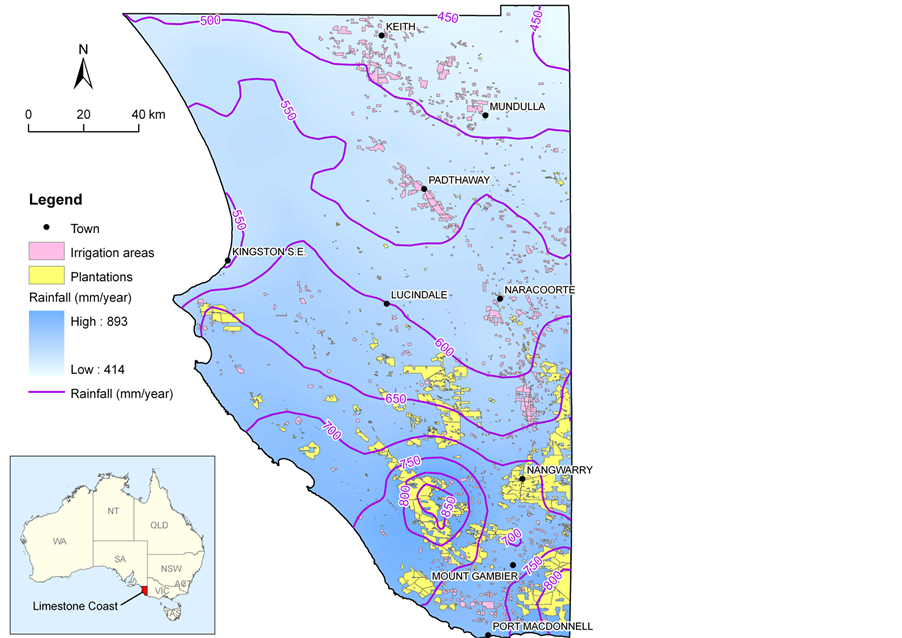
Figure 1. Limestone Coast location map and long term average (1961-1990) rainfall contours with current location of irrigation and plantation areas.
tion which will also affect the total availability of groundwater. The watertable over some parts of the region has declined over the last 30 - 40 years because of drier climate and groundwater extraction for irrigation. Uncontrolled developments of land use systems that reduce recharge and affect the availability of groundwater in the region is another issue in water management (e.g. expansion of plantation forestry). The challenge for the region is to develop an integrated water management regime at the system level that allows a balanced use of water resources taking into account the needs of all groundwater users within sustainable limits [1] . While there have been numerous studies on individual aspects of water balance; e.g. recharge [2] -[6] , plantation water use [7] -[9] , irrigation water use [10] -[14] , there is a lack of an integrated approach to water balance to compare the relative impact of water use components in the region.
Future intensification of agriculture is likely to rely on the availability of water of suitable quality, in localities of suitable climate and soils. A spatial analysis considering bio-physical factors for irrigation expansion (land suitability and water availability) in the region would help with the future planning of such expansions. Spatial multi-criteria decision making (MCDM) is a useful approach to serving this purpose. In general, a GIS-based MCDM involves a set of geographically defined basic units and a set of evaluation criteria represented as map layers. The problem is to combine the criterion maps according to the attribute values and decision maker’s preferences using a set of decision rules so as to rank each unit with an overall score. A number of spatial-based multi-criteria evaluation methods have been applied to land suitability assessment [15] -[24] . The application of advanced MCDM has shown to improve the credibility, transparency and analytic rigour of landuse and water management decisions [19] . Previous studies have assessed limitations of land for primary production in the study area [25] [26] ). However, the results are only useful to identify the factor which is the primary limitation in each mapping unit because the overall classification for a land was derived essentially based on the most limiting attribute and not considering the weight of individual attributes or evaluating the resultant uncertainties.
In this paper, we present current understanding of the water cycle in a regional water balance analysis as well as a multi-criteria analysis for future expansion of irrigation in the region as steps towards the development of an integrated water management regime.
2. Materials and Methods
2.1. A Conceptual Model of Hydrology and Control Volume
Many processes at different spatial and temporal scales affect the overall water balance of a hydrological system (Figure 2) including different land use activities (e.g. irrigation, forestry, dryland agriculture, water bodies, towns) with different water needs affecting the total water use as well as groundwater recharge occurring from the rainfall and irrigation. Drains play a role in collecting all the surface water as well as being fed by the deeper drains tapping into the groundwater, before flowing out to the sea. At the same time, exchanges between different aquifers take place, but they are not considered here for a regional water balance analysis.
In a water balance analysis, we must define the control volume and a time frame for which the calculations are carried out and assumptions are valid. The control volume, for this analysis, consists of the area from the surface to the watertable (the vadose zone) considering all flows occurring between this zone and outside the zone (i.e. fluxes to and from the groundwater, atmosphere, and the sea). The boundaries used for the water balance analysis are shown in Figure 1.
A simplified conceptual representation of the hydrological components of the water supply for the region is shown in Figure 3, following our understanding of the hydrological system in the region.

Figure 2. Schematic representation of the water cycle processes in the Limestone Coast.
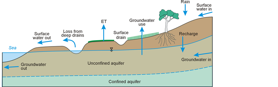
Figure 3. A simplified conceptual model of the hydrology Limestone Coast.
2.1.1. Regional Water Balance Analysis
A regional water balance can be written as:
 (1)
(1)
where Inflows refer to all incoming water to the region and Outflows refer to all the outgoing water flowing out of the system. ∆S refers to the change in the region water storage. When averaged over a long period, ∆S can be neglected (assumed zero).
At the regional scale, the main inflow is rain (P) which recharges (Re) the underground aquifer(s) as a proportion not being used for evapotranspiration (ET) of crops and natural vegetation or intercepted by trees and plants. Inflows also include surface inflows to the region (Qin) and groundwater pumped to the surface for use (GWuse). The Outflows consist of mainly the ET from different land uses as well as the flow of drains consisting of surface drains (Qo-s) and deeper drains collecting groundwater or fed by springs before flowing out to the sea (Qo-gw).
Equation (1) thus can be written as:
 (2)
(2)
The intention was to estimate an average annual water balance for the region within a period covering the years 1995 to 2004. Where data did not exist for some components, estimates based on assumptions about these average conditions were made (e.g. average land use). The steps followed for estimation of these components are described in the following sections.
2.1.2. Climate Data
Mean annual climate surfaces for 1961-1990, the reference period used by the Bureau of Meteorology, from QDNR (Queensland Department of Natural Resources) SILO daily data [27] were used for the analysis. The dataset provides interpolated data for a 5 km by 5 km grid across Australia. Areal potential evapotranspiration (ET0) data calculated from the QDNR gridded data set (daily temperatures and solar radiation) were used in the analysis. Using these climate surfaces, the long-term average rainfall and potential evapotranspiration for the region were calculated and scaled to the water accounting period using climate data for a few stations in the region [28] . For example, average annual rainfall and ET0 after 1995 were 95% and 98% of the long term averages. These figures were used to scale the long term averages to the period of our analysis.
2.1.3. Surface Water and Drains
The catchment contains a small number of well-defined flow paths that exist primarily as ephemeral creeks. All the data were obtained from the Department of Water Land and Biodiversity Conservation (DWLBC) surface flow archive (http://e-nrims.dwlbc.sa.gov.au/swa/map.aspx).
There are two types of drains flowing out to the sea: surface drains and ground water-fed system of drains which are deeper drains collecting groundwater or are fed by springs before they flow out of the region and to the sea.
2.1.4. Recharge to Groundwater (Re)
Here we refer to recharge as the water moving vertically through the soil, and adding to the groundwater storage. We used the mean annual values of recharge calculated by [6] and updated by [29] mostly with the watertable fluctuation method using the existing water level observation network. These values, ranging from 15 to 200 mm/year, are shown in Figure 4 for all groundwater management zones in the region.
2.1.5. Estimating Evapotranspiration (ET)
For estimating average annual ET in the catchment, land use data for the study area were categorised into 5 classes: irrigated areas, dryland agriculture, plantation forestry, natural vegetation and wetlands/water bodies. In the absence of actual ET measurements different methods of ET estimation were used for each class.
2.1.6. Irrigation Areas
For areas under irrigation, ET estimation requires specific crop water use (ETc) calculations. These were calculated mainly following FAO 56 methodology [30] which is based on the relationship between potential reference crop evapotranspiration (ET0) and a crop factor (Kc) as in Equation (3) (See [28] ).
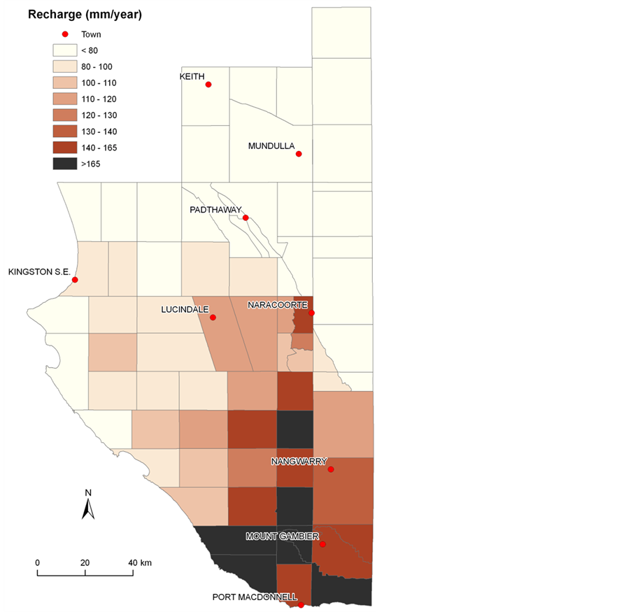
Figure 4. Recharge estimates of the region (Based on [6] and [29] ).
 (3)
(3)
Monthly ET0 values in mm were obtained from the climate data together with the information reported on land use and crop mixes under irrigation [10] -[13] to calculate ETc according to Equation (3). Monthly Kc values for different crops (mainly pasture, vines, lucerne, cereals, fruit, vegetables and potatoes) were taken from published values and local studies [14] [25] [31] . ETc values were converted to volumes (ML) of water considering the areas of crops in each year and averaged over the years of analysis.
2.1.7. Dryland Agriculture
For these areas, an estimate of ET was made based on average empirical values suggested by [32] based on the work of Fu [33] .
Actual evapotranspiration is calculated in the model using the following equation from [33] :
 (4)
(4)
where:
ET = actual evapotranspiration ET0= potential evapotranspiration P = rainfall w = a model parameter A single-parameter hyperbolic function (Equation (4)) interpolates between dry (rainfall limited) and wet (energy limited) total evaporation rates. The value of this parameter (w) describes the influence of catchment land characteristics and vegetation on actual evapotranspiration. In a water balance study of over 270 Australian catchments [32] , it was found an average value of 2.55 for w parameter to give good ET prediction (by Fu’s model) against the observed data. We used this average value in Equation (4) for ET estimation in dryland areas.
2.1.8. Plantation Forestry
An average area for forestry during the water accounting period was estimated as 110,000 ha. Water use by tree plantations in the region has been studied mostly on shallow groundwater areas and in closed canopy [7] [9] with a reported average water use of 944 mm/year. To consider an overall average water use (ET) by forestry, we need to take into account the relative areas on shallow water table (<6 m depth), the mix of different trees (pine plantation vs. blue gum) and the whole crop cycle water use (i.e. there are periods before canopy closure and after harvest). Based on these factors and previous experience, an average annual ET for the plantation forestry was estimated to be around 740 mm/year [R. Benyon, Pres. Comm.].
2.1.9. Natural Vegetation
There are large areas of land under nature conservation and natural vegetation. They are highly variable in vegetation composition, structure and spatial arrangement which are likely to affect their water use. For this land use we considered expert opinion on long term average water use of this natural vegetation to be almost the same as the average rainfall for the region [28] .
2.1.10. Wetlands and Water Bodies
For water bodies including lakes and reservoirs, Kc was assumed 0.7 and for the wetlands a value of 1.1 was considered for large wetlands [34] .
2.2. Spatial Multi-Criteria Analysis
A spatial multi-criteria assessment used here implements fuzzy quantifiers and analytical hierarchy process (AHP) in ArcGIS environment [35] . Topography, groundwater and landscape attributes and derivatives which affect irrigated landuse were selected as criteria and presented as spatial layers. The AHP was then employed to weight each criterion. The weighted averaging operator for selected values of fuzzy quantifiers was applied to derive several evaluation scenarios showing alternative potential suitability maps.
2.2.1. Suitability Classification
The suitability classes were adapted from the Food and Agricultural Organization system [36] . They consist of four levels describing land with high potential (S1) to unsuitable (N) as in Table 1.
2.2.2. Evaluation Criteria
Groundwater, topography, and soil landscape attributes, considered important in irrigation, were selected mostly based on the available spatial data which were collected and compiled in previous studies [37] [38] . The Fifteen attributes including groundwater salinity, depth to water table, salinity, susceptibility to waterlogging, susceptibility to acidity, inherent fertility, boron toxicity, sodicity, root zone depth, water holding capacity, surface condition, steepness, subsoil structure, surface rockiness and surface texture were considered [24] . They are further grouped into five categories/objectives: 1) waterlogging and salinity; 2) soil fertility; 3) chemical barriers to root growth: 4) soil depth and water storage; and 5) topography and soil physical conditions (Figure 5). The threshold values for each of the four suitability classes of most criteria were determined based on the synthesis of main irrigated crops in the region [38] . Criteria indicating the impact of groundwater salinity were based on the general distribution of groundwater salinity for the unconfined aquifer through the area and taking into account the soil salinity associated with groundwater [25] .
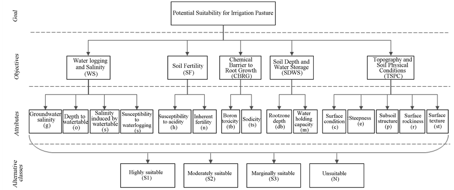
Figure 5. The hierarchical structure used in this study.

Table 1. Land suitability classification.
2.2.3. Criterion Maps
This procedure links the classified evaluation criteria to the spatial data. The original Soil Landscapes dataset is in vector format (polygon shapefile) [37] -[39] . Each polygon of the dataset is classified into four suitable classes. Where there are several land uses in a polygon, each with a different suitability classification, a single overall suitable class was identified based on the following two rules:
1) Assign a class level which represents the largest proportion of areas in the polygon;
2) Take the lower or lowest class level where multiple classes are contributing equally in a polygon (covering same proportions of the area).
All layers have four classes representing different suitability levels (Table 1) based on the threshold values assigned to them in Table 2.
In the study area, a key issue in the management of landuse and irrigation practices is to reduce accessions to the water table thus minimising the risk of waterlogging and salinisation due to rising water table levels. Therefore, two critical criteria from the Waterlogging and Salinity objective, groundwater salinity and soil salinity, were identified as key factors which constrain the expansion of irrigated pasture. These two spatial data layers were used as masks to exclude areas where groundwater or soil is classified as unsuitable before determination of criteria weights.
2.2.4. Criterion Weights
Criterion weights at both objective and attribute levels were derived using the pair-wise comparison which is the basic measurement mode of the AHP procedure. The procedure greatly reduces the conceptual complexity of a problem since only two components are considered at a time. This approach required the expert’s judgment for relative importance of one evaluation factor (objective and criterion) against another. The method employs an underlying semantic scale with values from 1 to 9 to rate the relative importance for two elements. The available values for the comparison are the member of the set: {9, 8, 7, 6, 5, 4, 3, 2, 1, 1/2, 1/3, 1/4, 1/5, 1/6, 1/7, 1/8, 1/9},
Table 2. Pair-wise comparison matrix of objectives and calculated weights.
with 9 representing absolute importance and 1/9 the absolute triviality [40] [41] . The comparison matrix at objective level is presented in Table 2 which assigns a numerical value showing relative importance of each objective. In this study, “Soil Fertility” objective has been regarded slightly more important than “Chemical Barriers to Growth”; hence a value of 2 has been assigned to the corresponding matrix position (Table 2). The transpose position automatically gets the reciprocal value, in this case 1/2. At the attribute level, a comparison matrix taking the same format of Table 2 was constructed for each of the objectives by comparing associated attributes. Based on these matrices, the relative weights for objectives and criteria were derived by a GIS-based model called FLOWA [20] [21] [42] .
2.2.5. Order Weights
After the weights related with criterion maps were input into the FLOWA, the module specified a linguistic quantifier to generate a set of weights, and therefore, computing the overall evaluation by means of the weighted averaging (OWA) combination function. Several resultant maps representing different scenarios were obtained. The suitability map, which was derived from the moderately optimistic scenario, was then overlaid by the current land use map. It was further compared with water availability data by excluding areas identified as having a negative water balance (i.e. groundwater over use or allocation) [29] to show the extent of potential areas for irrigation expansion.
3. Results and Discussion
3.1. Regional Water Balance
Calculations of recharge resulted in a mean annual volume of 1110 GL, while average rainfall was calculated as 11,942 GL. For the surface inflows, a total of 17.52 GL was calculated while the total outflow from the region consists of surface drains with total flow of 106,400 ML and groundwater-fed drains with total of 97,315 ML.
Annual ET estimates are summarised in Table 3. Dryland is by far the largest consumer of water (ET) of all land use classes (7687 GL). Total ET from irrigated land is estimated at 404 GL which compares reasonably well with the average reported irrigation water use in the region [43] of 448 GL which includes irrigation losses as well as ET. Considering all components of annual regional water balance comprising all water entering the surface (inflows) and leaving the region (outflows), Table 4 gives a summary of the water balance. The difference (balance) between inflows and outflows is relatively small (42 GL). This is equivalent to 0.33% water balance error. This, without considering uncertainties and some possible compensating errors, is an indication that the system overall is in balance and our estimates roughly describe the physical characteristics of the hydrology of the region.
The results show that a large proportion (90%) of all the water entering the region leaves the surface as evapotranspiration. Of the remaining water, 8.8% goes to the groundwater as recharge, while less than 2% leaves the region as surface water in drains or creeks.
Of the total annual evapotranspiration of 11,193 GL from the region, irrigation accounts for only 3.6% and plantation forestry for 7% total ET. Not all of this water use comes from the groundwater and in our analysis we have not separated the sources of water use (i.e. rainfall and groundwater).
Table 3. Average annual ET estimates from each land use type.
Table 4. Annual regional water balance components.
The average annual volume of water applied for irrigation is 400 GL/yr or 605 mm/yr which, when added to the average rainfall, yields a total of 1175 mm/yr. Based on the first order approximations, if only 630 mm/yr is evapotranspired from these lands, then the rest (545 mm/yr) is recharge. Thus, on average (across all soil, crop and irrigation system types) about half (46%) of the total water applied is returned back to the aquifer. This simplified analysis does however neglect the timing of rainfall, irrigation application, crop water use and fallow periods. In reality, a higher proportion of irrigation water returning to the aquifer will be expected under flood systems and lighter soils and much lower rates under more-efficient systems.
It should be noted that this regional (vadose zone) water balance gives an overall picture of the hydrology of the system without giving a balance of the groundwater. It also does not consider the spatial distribution of these components as they are averaged in space and time with rough estimates and assumptions. For a comprehensive and integrated approach for studying impact of different scenarios (e.g. climate, land use change) on water resource management, a fully dynamic model of the surface and groundwater of the region is needed which is beyond the scope of this study. Nevertheless, the water balance results when considered with the results of spatial analysis could help in better understanding of the system and making decisions on expansion of irrigation in the region.
3.2. Spatial Analysis
The resultant suitability map (Figure 6) shows the extent and distribution of the land suitability classes. There is about 13% (217,542 ha) of total area being classified as highly suitable (S1), while moderately and marginally suitable classes represent 42% (728,452 ha) and 5% (87,863 ha) of land respectively. The suitability map when overlaid with present landuse map (Figure 6) revealed that, in the study area, 25% (16,325 ha) of present irrigated land falls in the highly suitable class, while approximately 46% (30,265 ha) occurs in moderately suitable areas. There is only over 4% (2932 ha) under marginally suitable areas and more than 25% (16,755 ha) exists under unsuitable regions which consists of irrigated modified pasture, irrigated cropping (e.g. hay and silage) and irrigated perennial horticulture (e.g. vine fruits). They are mainly located in the north of the region where groundwater salinity is classified as greater than 2000 mg/L. Highly suitable land (S1) should be retained for irrigated agriculture since limitations to irrigated cropping in S1 land can be overcome by standard management practices. Policies should be considered which protect this land from unnecessary subdivision for urban or rural residential use or other uses such as roads. Limitations to irrigated pasture on moderately suitable land (S2) need

Figure 6. An evaluation map of irrigation suitability derived from WLC approach and overlaid with present landuse map.
to be recognised because a decline in productivity may occur and a range of landuse problems may develop if this land is used and managed inappropriately.
Currently, less than 8% of the total highly suitable lands have been used for irrigation practice. A large proportion of highly suitable land, located in the south part of the region in particular, has a great potential in cultivating more irrigated agriculture. However, not all suitable areas can be considered for irrigation
as groundwater resource is limited and its management and allocation planning has been the subject of many reports (e.g. [6] and [29] ). When water availability was considered as a limiting factor (Figure 7) where the groundwater allocation or use was larger than the recharge, the total highly suitable areas for irrigation expansion is estimated around 94,632 ha (S1 class) mostly around centre, south and western side of the region. In planning any expansion of irrigation areas, other important factors, such as economics and environmental aspects of such plans must also be considered. Future studies should also link a water balance analysis of land use change (i.e. crop-soil-water balance model) to a spatial multi-criteria analysis to enable estimation of future water use and recharge under proposed scenarios of irrigation expansion. A fully dynamic groundwater model could better describe the groundwater balance of each management zone for future scenarios. Such an analysis, when coupled with economic analysis, could give a more comprehensive view of the water cycle and its spatial distribution in the region for current and future water management planning.

Figure 7. Areas identified suitable for irrigation expansion considering water availability.
4. Conclusions
At the regional level, our analysis showed that a substantial (~90%) part of the water input to the region is consumed through either plant transpiration or evaporation from water bodies, wetlands and soils. Irrigation only contributes to about 4% of this total ET, though it consumes a substantial part of the groundwater extraction in the region. Plantation forestry is considered as a “water use” activity and its share of the total regional ET is around 7%. Around 9% of the total rainfall is recharged to the aquifer and is the major contribution to this huge groundwater resource while less than 2% leaves the region as surface water in drains or creeks.
The regional water balance gives an indication of the relative contribution of different components of the water cycle at the system level and as such it does not show the spatial and temporal variability of these terms.
A spatial fuzzy multi-criteria evaluation approach has been applied for spatial suitability assessment for irrigation. The resultant evaluation has revealed that about 70% of existing irrigated cropping is located in highly suitable and moderately suitable lands in the eastern half of the region. But vast areas of highly suitable land exist where irrigation can be expanded. Expansion in irrigated agriculture is likely to present new demand for water resources and as such, the availability of groundwater in potential suitable areas should be considered when planning for expansion. When areas identified as water limited were excluded from the potential suitable areas, the total highly suitable areas for irrigation showed a maximum of 94,632 ha distributed mainly in the center, south and western part of the region. The resultant potential irrigation maps are intended to provide a regional view of areas potentially suitable for irrigation. Future planning should consider water balance changes resulting from land use change (through modeling) as well as economic and environmental assessment of future land use scenarios.
The use of a multi-criteria evaluation model in this study showed some advantages over the conventional methods as it avoids arbitrary decisions on assigning related weights to the criteria. It allows exploring and visualizing a wide range of different multi-criteria decision strategies. When (in future) linked to water balance models, it would facilitate a better understanding of the patterns of alternative land use and could give a comprehensive picture of irrigation land use impact on future water resources management and development planning.
Acknowledgements
This work has been carried out as part of a suite of activities funded by the Cooperative Research Centre for Irrigation Futures (CRC IF) in the Systems Harmonisation Program. The funding of the CRC IF is gratefully acknowledged. We also wish to acknowledge those who have provided inputs to this study. In particular we acknowledge: DWLBC staff at Mt. Gambier for providing spatial data, information and reports.
Drs. Richard Benyon and Judy Eastham (former CSIRO) for providing insight to the estimation of water use by plantation forestry and natural vegetation and Mr Peter Briggs (CSIRO) for providing long-term climate surfaces (rainfall and potential ET) and Mr Heinz Buettikofer (CSIRO) for the graphics and GIS support.