UV Index Modeling by Autoregressive Distributed Lag (ADL Model) ()
1. Introduction
The modeling of Ultraviolet Radiation (UV) and its index (UV Index or UVI) is important, among other reasons; due to lack of information on these variables and small number of stations [1] -[3] . This fact leads researchers to invest in development of computational, physical, statistical and stochastic models to estimate or forecast/projections of UV/UVI [4] [5] .
In Brazil, some statistical models for UV-UV Index were validated and performed by researchers [6] built statistical models and artificial neural networks to estimate UV and obtained a mean square error of less than 5%. Researchers of Center for Weather Forecasting and Climate Studies, National Institute for Space Research (INPE/CPTEC) [7] conducted a study on the estimates of the radiative transfer model UVSIM (Ultra-Violet SImplified Model) to analyze the effect of cloud in UV Index. The results showed a high correlation model (0.8) with observed values. In this model, the input parameters are the coordinates of UVSIM time (hour, day), geographic (latitude, longitude), cloud cover and Ozone concentration estimated by instrument OMI (Ozone Monitoring Instrument) of satellite AURA/NASA. Finally, the model UVGAME (UV Global Atmospheric Model) was used in research on the UV Index variations and regional and seasonal distribution of the number of cases of skin cancer in the Brazilian’s skin color [8] .
Internationally, the historical anthropogenic changes in the surface all-sky UV-B radiation through 1850-2005 are evaluated by analyzing the CMIP5 transient historical simulations performed with MI-ROC-ESM-CHEM were the researchers studied [5] . The results of the study have indicated that changes in ozone transport in the lower stratosphere, which is induced by increasing greenhouse gas concentrations, increase ozone concentration in the extra tropical upper troposphere and lower stratosphere. These transient changes work to decrease the amount of UV-B reaching the Earth’s surface, counteracting the well-known effect increasing UV-B due to stratospheric ozone depletion, which developed rapidly after 1980.
The research [9] conducted an analysis by 13 models used in prediction schemes for UV Index, including simple regression. The models had parameters like location data, Total Ozone column and solar zenith angle. The authors considered that the differences between the models were derived from treatment of unknown input parameters, especially aerosols. Another research [4] used data from the period 1976-2006 and a regression model to establish a statistical relationship between UV and content ozone, global solar radiation and cloud cover at different scales of time and explanatory variables in order to reduce the standard error. Others Researchers [10] established a statistical relationship between Total Ozone, solar zenith angle and UV irradiance. Modeling of UV and problems on the radiative transfer in clear and turbid environments were described by [11] . The researchers of European Communities [12] emphasizes that prediction methods vary in simple statistical methods used to certain times and local until robust methods to forecast some hours to several days, either for all sky or clear conditions sky. The accuracy of forecasts of UVI is mainly limited by the quantity and quality of input data. Finally, [12] explains that in future the data assimilation of large-scale ground-based observations of Total Ozone, aerosol and cloud cover through satellite should considerably improve accuracy for models.
This study presents the proposal to apply an autoregressive distributed lag model (ADL) or Dynamic Linear Regression model. This is a linear regression model involving time series that includes current and past values of the variable under study and explanatory variables with or without time lags [13] [14] . It is used when there is a dependency structure between these variables. These models have been used in the past in the environmental field [15] and dynamic regression models are widely used because they express and model the behaviour of a system over time [16] . As the variables of the model are indexed by time and since there are lags in both exogenous and dependent variables, then the ADL model should be used [15] .
The ADL model can be well utilized to make forecasts/projections (extrapolation). In this study, UV Index is response variable and Total Ozone is explanatory variable. It is worth noting that the more current information is of greater importance to improve forecasts [17] .
The modeling of UV/UV Index and its use for forecasts/projections is important due to increase in Flow of Ultraviolet Radiation (FUV) on the surface of the Earth. Researches [18] -[20] have warned of an increase in biologically active ultraviolet radiation (erythemal dose) due to decreasing levels of stratospheric ozone.
Ozone is the component responsible in absorbing the UV in earth’s atmosphere, preventing it to come fully to the surface of the Earth. The reduction in the quantity (Total Ozone column or Total Ozone) is the main cause for the increase of UV and brings impacts on nature and human health [8] [20] [21] . The Global Total Ozone average from 2005 to 2009 is around 3.5% below that recorded in the period 1964-1980. The changes in this variable occurred since 1970 (base year) to 2010, in which there is a reduction of 3% [20] [21] .
The researchers [22] analyzed the effects of climate change on the ozone layer using climate models. The models indicated an accelerated circulation in the stratosphere with changes in the spatial distribution of tropospheric and stratospheric ozone. The authors showed that, in future scenarios of the IPCC (until 2095), the UV Index would change with clear skies, with a 9% reduction in high northern latitudes and increases of 4% in the tropics and up to 20% at high latitudes of the south, during late spring and early summer. The results suggest that climate change will alter the balance of tropospheric ozone and UV Index, which would have consequences for radiative forcing in the troposphere, air quality and human health and ecosystems, however the amount of ozone in the atmosphere is recuperating as the result of the Montreal Protocol, in force since 1989 [21] -[23] .
In Northeast Brazil (NEB) there is an increase of Flow Ultraviolet Radiation (FUV) [16] . This fact has motivated this study, whose goal is to build a forecasting model of UV Index in city of Natal, capital of state Rio Grande do Norte, located in the NEB.
This article aims to conduct modeling, using ADL model, for variability of UV Index in city of Natal, east coast of the Brazilian Northeast, a function of Total Ozone and perform predictions (interpolation), forecasts/ projections (extrapolation) and trend analysis, collaborating to understand the issues presented.
2. Material and Methods
2.1. Study Area
Natal is a tourist town with beautiful beaches and 853,928 inhabitants [24] located in east coast of NEB between the sea (South Atlantic) and the right bank of the Potengi River near the equator (5˚45'54''S and 35˚12'05''W). The city is called by its inhabitants of “Sun City” [25] due to the great sunlight related to the intensity of solar radiation and total annual insolation of 2968.4 hours [26] . The “Sun City” has problems of non-melanoma skin cancer rates above the regional average for women (54%) and men (87%) [27] .
In this city the UV Index is classified as “extreme” from October to April and “very high” from May to August. The annual variability has a characteristic in September and October that consists of stabilization and reduction in UV Index because of highest concentration of Total Ozone and increased presence of marine aerosols [28] . The annual UV Index average observed for the period was 11 (±1.0). In the daily cycle, the maximum UV Index occurs around 11:20 am, classified as “high” starting from 9:00 am local time (time zone GMT-03) to 10:00 am achieves intensity considered “too high” [29] .
2.2. UV Index-Formulation
The UV Index describes the intensity of UV in relation to its photo-biological effect [1] being defined by equation (1):
 (1)
(1)
in which Eλ is the spectral irradiance expressed in W×m−2×nm−1 to the wavelength λ and dλ it is the wavelength range used in the integral calculus. Ser is the reference action spectrum erythema and Ker is a constant equal to 40 m2×W−1.
The UV Index was proposed by the World Health Organization (WHO) [1] based on the reference spectrum of action erythema of [30] .
2.3. Data for UV Index and Total Ozone Column
The daily data (2001-2012) of UV Index were measured in the surface by: 1) Radiometer GUV (Ground-based Ultraviolet Radiometer) [31] installed in Laboratory of Tropical Environmental Variables of National Institute for Space Research/Center Regional of Northeast (INPE/CRN/LAVAT) and 2) Sensor Model UV-6490 of Meteorological Station Davis installed at the Laboratory of Hydraulic Machines and Solar Energy in Technology Center of University Federal of Rio Grande of Norte (UFRN/LMHES). The daily maximum of UV Index was collected on interval of 11 h - 13 h, independent of sky conditions A set of daily data (2001-2012) of Total Ozone (DU units) was collected at TOMS (Total Ozone Mapping Spectrometer) e OMI (Ozone Monitoring Instrument), available in http://avdc.gsfc.nasa.gov/. The spectrometer TOMS is atmospheric sensor has been flying on different missions within NASA’s Earth Probes Program. The objective is to extend the global ozone data set that began in 1978 with the flight of TOMS on NIMBUS-7. The end of the operation occurred in 2005 when he worked on the platform Terra Probe [32] . The instrument OMI was launched in July 2004 on board EOS-Aura. OMI monitors the recovery of the ozone layer in response to the phase out of chemicals, such as CFCs. Together with its companion instruments MLS and HIRDLS it will measure criteria pollutants such as O3, NO2, SO2 and aerosols [33] .
2.4. Completing the Missing Data
The presence of missing data on UV Index series and the need to complete time series for stochastic models was applied multiple imputation technique for each group of same month, using Predictive Mean Matching method (PMM) [34] [35] placed in MICE package (Multivariate imputation by Chained Equations) in the R software free, available at http://www.r-project.org/ [36] . The software MICE used allowed program their own imputation function, while at the same time it supports a variety of imputation methods [37] .
The PMM method is an imputation method that combines parametric and nonparametric techniques. It imputes missing values by means of the Nearest Neighbour Donor where the distance is computed on the expected values of the missing variables conditional on the observed covariates, instead of directly on the values of the covariates [38] . The PMM is a variant of linear regression that determines an imputed value calculated by the regression model closest to the observed value [39] [40] . The PMM consider the following formulation (equation (2)) for each i missing in Y
 (2)
(2)
Consider X a variable without missing data,  the group of observed values; and
  , one obtains Ŷobs found as the nearest observation
  .
.
There are a number of imputation methods: simple imputation methods, regression imputation, hot deck imputation methods and distance function matching. PPM method is considered to be the most accurate, since it combines elements of regression, nearest-neighbor and hot deck imputation [41] and is characterized as a general purpose method [42] .
PPM can overcome the difficulties of both parametric and nonparametric imputation techniques, given the fact that parametric techniques may fail when the model is not suitable for the available data and nonparametric techniques require high amount of observations [38] .
The PMM application results were promising for monthly scale when compared with the original data [43] [44] , although performance of the predictive mean method varies considerably with the predictive power of the imputation regression model and the percentage of cases with missing data on income [45] .
The procedures for filling the missing values using the method of PMM must follow the criteria: data are monthly and the regression model was applied to each group of same months (same name) of full data series [39] [40] , because the use of locally adjusted PMM method provides reduced bias [46] .
2.5. Autoregressive Distributed Lag Model (ADL)
The ADL is a parametric model that combines the dynamics of time series and the effect of explanatory variables. It consists of stochastic regression involving time series that includes current and past values of the variable under study and explanatory variables, including lags [13] [14] [47] . This model uses the notation ADL (pj, p), wherein pj and p indicate the lag order of the variables or variable, respectively, dependent and independent [14] . General representation of the model is defined by equation (3):
 (3)
(3)
in which: yt: dependent variable in time t; β0: a constant; yt‒i the dependent variable in t ‒ i; xjt‒i is the jth independent variable in t ‒ i, by i = {1, ×××, pj} e j = {1, ×××, p}; βji: coefficient of the jth independent variable in t ‒ i; fi: coefficient of the dependent variable in t ‒ i; εt random residual [13] [14] [48] .
The method of Ordinary Least Squares was used to estimate the parameters in the model: β0 representing the intercept and β1, β2, …, βn are the angular coefficients [49] [50] . In the model proposed in this study, yt refers to UV Index at time t and xt was considered the Total Ozone at time t.
In applications of ADL model, the residual error must meet the following assumptions: the errors εt are random and independent variables following a normal distribution: εt ~ N (0, σ2) with zero mean, and constant variance (σ2) (homoscedasticity) [51] . The Kolmogorov-Smirnov and Shapiro-Wilk tests were used to verify the normality assumption [52] . The homoscedasticity assumption was measured using the Breusch-Pagan test [53] [54] .
The F test was used to test the significance of the regression equation and t-test to measure contribution of explanatory variable [55] [56] . In this study was applied 5% significance for the tests.
There are a number of distributed lag models and the selection of the appropriate one consists in specifying the lag length correctly [16] . The ADL model includes lagged values of both independent and dependent variables and was chosen due to the fact that: 1) it is not so strict, as geometric lag models or finite distributed lag models and 2) it is a general form that can capture the current and lagged effects of an independent variable over the dependent [16] .
In this study the Cross-Correlation Function (CCF) was used to determine the number of lags between UV Index and Total Ozone for considered on the ADL model [57] [58] . The autocorrelation function (ACF) was applied to the original series of variability of UV Index in order to verify the seasonality and non-stationarity this series [58] .
Box-Pierce test [59] and Durbin-Watson test [60] [61] were applied to assess the independence of errors.
The calculations and results were obtained through the procedures performed by the R software free [62] [63] and package dynlm (Dynamic Linear Models and Time Series Regression) authored by [64] .
2.6. Trend Analysis
The Mann-Kendall test nonparametric [65] was applied with 95% statistical significance to analyze the trend of the number and intensity of UV Index. This test compares each value of the temporal series with the remaining values in sequential order, counting the number of times that the remaining terms are greater than the analyzed value [66] . This test is the most appropriate method to analyze weather tendencies in climatological series and has been used to calculate climatic tendencies [67] -[69] . In applying the Mann-Kendall test, we used the package SeasonalMannKendall (Mann-Kendall trend test for monthly environmental time series) in library of software R [70] [71] .
3. Results and Discussions
3.1. Descriptive Study
The variability and monthly and annual average of UV Index and Total Ozone are presented in Figure 1 and Table 1. The average annual of UV Index is 11 and for Total Ozone are 264.8 UD. The colors in the graph of UV Index are associated with the categorization of risk of the WHO. The UV index reaches the value classified as “extreme” (color violet) in seven months of the year, between spring and summer.
The annual variability of the UV Index in city of Natal has a stabilization/reduction in September e October as associated with a higher ozone concentration [28] . This feature was observed in this data series, as shown in Figure 1.
3.2. Completing the Data Daily of UV Index.
There missing data in 13 months of the total of 144, corresponding to 9.03% of the total number of observations. The process of multiple imputations through PMM was used to completing the missing data. The Figure 2 shows the time series of UV Index with data filled by method PMM and Total Ozone (simultaneously).
In the series very high UV Index values were observed in three periods, February 2005 and 2007 with 13.7 (252.6 DU) and 13.5 (250.5 DU) respectively and March 2010 with 13.6 (248.4 DU). The high values were coincident with low levels of Total Ozone. This study did not assess the causes of the extreme values of UV Index, however in Figure 2 identified that the low values of Total Ozone was associated with these measures.
3.3. Modeling in UV Index
The ADL model final was adjusted with historical values (period 2001-2011) of UV Index considering a lag 1, 4, 7 and 12 to capture seasonality. The signal of Total Ozone (explanatory variable) was used without and with lag 2. This ADL (4, 1) is represented by coefficients in Table 2.
The significance of regression equation was confirmed through of F test (F = 80.61 and p-value < 0.001).
A regression model is accepted if the residuals are standardized and homoscedastic. The Figure 3 shows graph

Figure 1. Boxplot by variability of the monthly UV Index and Total Ozone to Natal-RN for period 2001-2012. Source: INPE/CRN-LMHES/UFRN and TOMS-OMI/AURA.

Table 1. UV Index and Total Ozone in the city of Natal (monthly and annual average for 2001-2012).
Source: INPE/CRN/LAVAT-LMHES/UFRN and TOMS-OMI/AURA.

Figure 2. Time series of UV Index X Ozone total (vertical lines in green) for period 2001-2012 in city of Natal-RN.
Table 2. Coefficient regression (Coeff), standard error (SE) and p-value for ADL model.
of residuals (on top) and graphs for analysis of variance and normality. The normality of residuals was confirmed by Kolmogorov-Smirnov test (KS) (p-value = 0.76) and by Shapiro-Wilk test (SW) (p-value = 0.40).
The Breusch-Pagan test (p-value = 0.86) confirmed the hypothesis of homoscedasticity of residuals. The Box-Pierce test indicated independence of residuals (p-value = 0.07) together with Durbin-Watson test (p-value < 0.001).

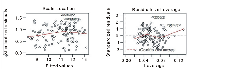

Figure 3. Graphs for diagnostic of residuals of model ADL (4, 1).
3.4. Validation of Model ADL
The Figure 4(a) shows the UV Index observations and predicted values (interpolated) for the years 2002‒2011 by the model ADL.
The ADL model presented good results for the interpolation with a mean squared error (MSE) of 0.36 and correlation of 0.90 between the interpolated data and observed of UV Index and MSE of 0.30 and correlation of 0.91 for extrapolation (forecast to 2012) in Figure 4(b). These results were considered appropriate and validated the model to make forecasts.
3.5. Trend Analysis of UV Index and Total Ozone.
The trend study for UV Index and Total Ozone in observed period occurred through the Seasonal Man-Kendall test. Was identified stability in UV levels (τ = −0.009 and p-value = 0.896) and a downward trend in the levels of Total Ozone (τ = −0.302 and p-value < 0.001). The Figure 5 shows the time series with lowess smooth.
The projection performed by model for a period climatological (2012-2042) indicated a trend of increased of
 (a) (b)
Figure 4. (a) UV Index data observed (black) and prediction or interpolation (blue) for the ADL model for the city of Natal for period 2001-2011; (b) Observations of UV Index (red), interpolation data by model (black), forecast values for 2012 (blue) and confidence interval (orange).
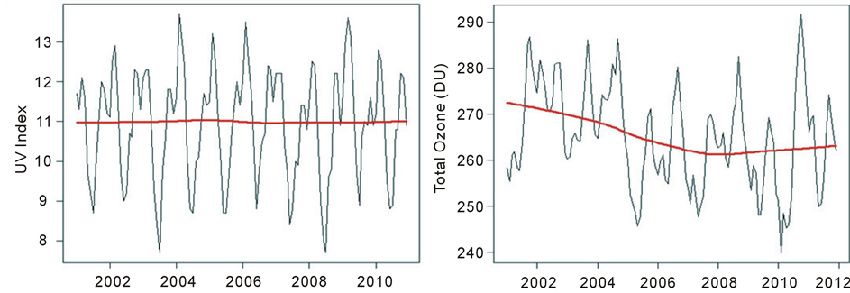
Figure 5. The time series plot with lowess smooth for UV Index and Total Ozone for the period observed.
UV (τ = 0.955 and p-value < 0.001) whereas Total Ozone remain on this trend. The current average annual of UV Index is 11.0, however the model predicts a rise in 2042 for average of 11.8, an increase of almost one unit of the UV Index. At present the amount of ozone in the atmosphere is recuperating [2] [5] and must change this trend.
4. Final Considerations
In constructing the model ADL (4, 1) have been found MSE and correlation index between UV index data (interpolated and extrapolated X observed) considered appropriate to validate the model. Furthermore, in model we confirmed that residues were random variables with zero mean, independents, normalized and with homoscedasticity, fact that can provide errors in estimates of regression coefficients and the general applicability of the model if not confirmed.
In the study, the UV Index model was built with a single explanatory variable, the Total Ozone along with the autoregressive signal of UV index. This is characteristic of ADL model which can combine the autoregressive signal and explanatory variables with the possibility of introducing lags.
The forecast/extrapolation performed by model for a climatological period (2012-2042) indicated a trend of increased UV (Seasonal Man-Kendall test scored τ = 0.955 and p-value < 0.001) if the Total Ozone remain on this tendency to reduce. In those circumstances, the model indicated an increase of almost one unit of UV index to year 2042.
Finally, it is noteworthy that there is a scenario of increased the UV flux at Earth’s surface, being relevant the development of forecast models to UV index which can collaborate on preventive actions against high rate of cases skin cancer in northeast of Brazil.
Acknowledgements
This work was supported by the CNPq, National Council for Scientific and Technological Development, Brazil: via the Doctor Sandwich—SWE/CsF (246611/2012-0) and projects “ATMANTAR”-MCTI/PROANTAR/CNPq (520182/2006-5) and “A Atmosfera Antártica, Conexões e Impactos Ambientais na América do Sul”, INCT-APA, MCTI/PROANTAR/CNPq (574018/2008-5).
The author thanks the State University of Bahia by financial support during the PhD of PPGCC/UFRN and to Federal Institute of Education, Science and Technology of Bahia by study leave.