Keywords:Jumps, Euribor Interest Rates, Poisson-Gaussian Model, Negative Surprises

1. Introduction
“…I think that the Maastricht Treaty and the launching of the ECB were a magnificent success and I think that when you go back to the Delors Report in 1989, it was quite remarkable when that came out, because it was a proposal for a single currency monetary union. It would have been much easier to have an 11 or 15-currency monetary union, but a single currency monetary union was quite a big step, and for a long time I thought that that was too big a step, that European governments would not be willing to accept it [the loss of sovereignty]. But the Delors gamble, and I think it was a big gamble, turned out to be successful and in retrospect, Europe is lucky that it ended up in that direction, rather than with an alternative” [3] . International Monetary Policy after the Euro (2005, page 48).
In accordance with the previous speech, it seems that searching for a convincing explanation to the ECB’s decisions announcement concerning the interest rate is an important subject especially when we find that the literature on the ECB interest rate market has not yet covered many specific aspects studied in the euro area.
Few works are presented in literature dealing with jumps in the Federal Fund rate in general and the EONIA in the eurozone. According to the advancement of [1] [4] -[10] , we remark that different analyses of Fed Funds in the United States are much wider than the study of EONIA in the eurozone where most studies have concentrated on finding whether the instruments and procedures to implement the monetary policy have repercussion on the overnight rate. [11] studies how the operational procedures and intervention forms of the central banks affect the characteristics and behavior of the one-day rate in the most industrialised countries (Eurozone and G7). [12] models the problem of the intertemporal decision in the reserve market, both for the central bank and for commercial banks.
[13] tests whether there are statistical differences in the behavior of the daily rate before and after the European Monetary Union (EMU), presenting a model for liquidity shocks focused from the demand side. [10] asserts that the timing of jumps is deterministic and coincides with the exact dates of the ECB’s meetings.
Our empirical analysis is implemented through a linear model that incorporates a fluctuation’s component. The resolution method for a linear interest rate differential equation will be obtained through a Poisson-Gaussian analysis. In this study, we aim at strengthening conclusion taken through a distinguished comparative analysis between a pure Gaussian distribution and Gaussian-Poisson process. Thus, we treat the information surprises result in discontinuous interest rate to quantify the effectiveness of the European Central Bank announcement channel. We choose as a reference the interest rate for interbank deposits in the euro zone determined as a 15% trimmed average of the interest rates contributed by the “Panel banks—banks with the highest volume of business in the euro zone money market”. It is also the rate at which a prime bank is willing to lend funds in euro to another prime bank. The EURIBOR is computed daily for interbank deposits with a maturity of one week and one to 12 months as the average of the daily offer rates of a representative panel of prime banks, rounded to three decimal places1.
This research examines the role of jump-enhanced stochastic processes in modelling the Euro interbank offered rate for different maturities. The paper offers four distinct sets of contributions. 1) We develop an analytical modelling framework for jumps in fixed income country. 2) We establish a Poisson-Gaussian model, and then deduce a pure Gaussian model. 3) We implement a comparative analysis for these models to detect limits and benefits for each one. 4) We determine which day can optimize the effectiveness of the ECB announcement channel.
The paper proceeds as follows. Section 2 deals with methodological aspects. Section 3 discusses the optimal period for estimation. Section 4 deals with the empirical results, we present those obtained through PoissonGaussian model and pure Gauss model (Section 4.1), then we present a method to extract day of the week effect recognition (Section 4.2). Section 5 summarizes and provides concluding remarks.
2. Methodological Aspects
Stochastic processes governing interest rates analysis is harder than that usually encountered for resolving equities and exchange rates. This complexity is due to mean reversion in models saving a surprising element with higher fluctuations. There are also very limited solutions for the stochastic differential equations. In this section, we present methodological aspects for our econometric specifications.
The mean reverting process for the interest rates can be written as:
 (1)
(1)
where  is a central tendency parameter for the interest rate r, which reverts at rate I. Therefore, the interest rate evolves with mean-reverting drift and two random terms. The former is propagation and the latter is a Poisson process embodying a random fluctuation f. The coefficient’s variance of the propagation is
  and the arrival of dynamic fluctuations is dominated by a Poisson process p with arrival frequency parameter h, which plots the number of deviations per year. The fluctuation means a possible rise or fall in the interest rate. Despite, these two repatriations, we will be able to attribute a constant value for each situation or to attribute a possible probability distribution.
Being at time t = 0, and looking ahead to time t = T, we are interested in the distribution of r(T) given the current value of the interest rate . In order to derive the T-interval characteristic function
  for the process (1), (
 is the characteristic function parameter).
 (2)
(2)
where , joining the complex formality. From (1) and (2), a third equation can be written as:
 (3)
(3)
where  comes from the effect of the Poisson shock [14] .
Illustrating the solution for the previous equation, we find that:
 (4)
(4)
Next, we can deduce the moments and the probability density functions for any choice in distribution where the rises or fall do not depend on the state variables.
Let  denote the nth moments, and
  be the nth derivative of
  with respect to
 , i.e.
 . Then,
 . Likewise
  denotes the nth moment of the shock (rise or fall).
  are the nth derivatives of K and L, respectively, with respect to
 .
.
 (5)
(5)
Then,
 (6)
(6)
We can also compute the first, second and third derivatives of K evaluated at , which are:
 (7)
(7)
Using the fact that , we obtain:

And the derivatives of L with respect to :
:

Then, we can write the intermediate value as:
 (8)
(8)
We can now write the analytical expressions for the moments:
 (9)
(9)
In discrete time, we express the process in Equation (1) as follows:
 (10)
(10)
where  is the daily variance of the Gaussian shock, and
  is a standard normal shock term.
  is the rise or fall shock, which is normally distributed with mean
  and variance
 .
.  is the discretetime Poisson increment, approximated by a Bernoulli distribution with parameter
 ;
;

Let  is distributed binomial being the sum of independent Bernoulli variables.
For x occurrences,


Under this expression, we have to classify the movements of possible fluctuations. The assumption made here is that we are searching for a jump, in each time interval either only one jump occurs or no jump occurs. Searching for a fall, in each time interval either only one fall occurs or no fall occurs. But the question that we will try to answer after the estimation is that: Does no jump mean necessary a fall or something else? According to [15] , this is tenable for short frequency data, and may be debatable for data at longer frequencies as it is the case in our paper. Since the limit of the Bernoulli process is governed by a Poisson distribution, we have approximated the likelihood function for the Poisson-Gaussian model using a Bernoulli mixture of the normal distribution (see Equation (10)).
Allowing the variance  to be ARCH in extending the Poisson-Gaussian model, the intensity fluctuation to depend conditionally on various state variables, the transition probabilities for the interest rate following a Poisson-Gaussian process are written as:
 (11)
(11)
In this equation noted (Equation (11)),  is an approximation measure of the true Poisson-Gaussian density with a mixture of normal distributions. It is worth noting that our estimation exercise uses Poisson-Gaussian models extended for ARCH effects. They allow for mean-reversion in fluctuations processes, and also test for the impact of the European Central Bank actions.
Designing by:

(Equation (11)) can be rewritten as:
 (12)
(12)
Searching for a pure Gaussian process, we attribute a null value to . Then, we obtain:
 (13)
(13)
Consider a Poisson probability density function , for a fixed but unpredicted signal, s, in the presence with a known background with mean
 .
.
Two values  and
and  are found for each value of s:
 (14)
(14)
where Q denotes the confidence level. Graphically, upon a measurement,  , the confidence interval
  is determined by the intersection of vertical line drawn from the measured value
  and the boundary of the confidence limit.
From Equation (12), a further Equation (15) is deduced as:

According to [16] , one of the valuable modifications addressed to the classical method of constructing confidence belts is:
 (16)
(16)
Our estimation involves maximizing the function L, where
 (17)
(17)
This may be written as:
 (18)
(18)
Consider a probability function of  that encompasses a set of parameters
  and N independent observations. Le Likelihood, L, is defined as
 (19)
(19)
From (19), the Equation (17) becomes:
 (20)
(20)
The same for (18):
 (21)
(21)
According to [17] and [18] , maximum likelihood estimators are usually biased. But the bias is zero in the asymptotic  limit, when the likelihood function becomes Gaussian and the standard deviation of
 , can be obtained from [19] as:
 (22)
(22)
If the large-N limit has not been reached, the standard deviation can be estimated by finding the value of  for which logL drops by 1/2 from its maximum at the optimum value
 .
.
The standard deviation will be symmetric with respect to  in the large-N limit.
For each process, we obtain estimates that are consistent, unbiased and especially efficient attaining the Cramer-Rao lower bond due to the satisfaction of the technical regularity conditions stated in Cramer [20] . This is in concordance with the efficient market hypothesis. Moreover, this justifies the application of the maximum-likelihood and thence the likelihood ratio test to this model. The constraints are that the weights for each sign of fluctuation (positive vs. negative) add up to one, which is already imposed in the equation above and that possible values of q are included in interval (0,1).
Given the analogy of this distribution to that of mixture distributions presented in Equation (11), ML is directly achieved as a solution to a system of first order conditions  as seen in [8] . Estimation is undertaken due to E-M algorithm of [21] .
3. Data Selection
Before To avoid any unfavourable event that would bias the result in favour of finding jumps, we eliminate some critical dates (negative surprises) collected from the financial times [22] .
First, before Wednesday 21 March 2001, the ECB had insisted that the US slowdown was unlikely to have much impact on Europe and therefore the interest rates would not change. Second, on Wednesday 21 March 2001, the ECB president (Duisenburg) said during a business school meeting in Germany that the ECB might need to consider cutting interest rates because the slowdown in growth in the USA may be stronger than earlier expected. Third, on Friday 23 March 2001, Statements of the Governor of the France ([23] ) and the ECB Chief Economist ([24] [25] ) indicated that the ECB would soon cut interest rates. Fourth, on Wednesday 4 April 2001, the ECB President and other members of the Governing Council all made statements that the ECB remains in a “wait and see” position. However, efforts ran into fresh trouble when it emerged that the governor of the Banque de France, has made a public council statement based on Thursday’s meeting without forewarning at least some of his colleagues. Fifth, on Tuesday 10 April 2001, Didier Reynders, the Belgium minister of finance and leader of the Eurogroup of finance ministers said: “We are still worried about the general economic trends and against that background everyone will have to take his or her responsibility… We will report the concerns about economic slowdown for the ECB to draw its own conclusion” This was also stressed by several commercial banks expecting a cut of European interest rates. The last event that we eliminate was on Wednesday 11 April 2001, where the ECB keeps interest rates on hold. The ECB disappointed governments, business, trade unions and the IMF, by refusing to cut interest rates and giving no sign that it would change its mind in the immediate future.
This section analyses the EURIBOR interest rate sample of 1945 daily observations over the period from January 1999—the starting date of Stage Three of the EMU—to February 2007 except some dates cited previously. The data is daily on frequency.
As
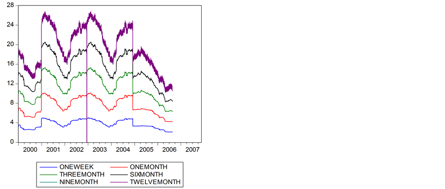
Figure 1.Evolution of the euro interbank rate for different maturities.
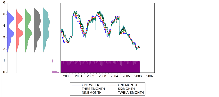
Figure 2. Kernel density spreading.

Table 1. Descriptive Statistics Euribor.(R1>)
Table 2. Descriptive Statistics (first difference of Euribor) R2 (ΔR1) .
Figure 1shows the fluctuations in the euro interbank rate and Figure 2 exhibits the kernel density repatriated for different maturities. They reflect liquidity conditions that are temporarily relaxed or restrictive on the money market. These fluctuations and the peaks are mainly related to the calendar effects and the fortnightly meetings of the Governing Council of the ECB.
When we observe Figure 1 and Figure 2, however, we can see a small lag during 2001 between trends in interest rates and the tone of statements. Note that as soon as early 2001, the markets were expecting a rate cut by the ECB. Nevertheless, the ECB did not change its key interest rate in February, March, or even in April 2001, whereas the economic slowdown seemed to justify a rate cut2.
Table 1 and Table 2 deal with descriptive statistics of the daily rate  and its first difference
  respectively over the period January 1999 to February 2007 except some critical days. Mean denotes the sample arithmetic mean, Median is the sample median, Max and Min stand for maximum and minimum respectively, Std denotes standard deviation and Skew and Kurt stand for skewness and kurtosis respectively. It is worth noting that changes in interest rates demonstrate considerable skewness and kurtosis. According to [26] , the presence of leptokurtosis in interest rate fluctuations is undeniable and jumps may explain the high degree of curvature in yield curves. Euribor interest rate volatility is very high, and persistent. This aspect is taken into consideration by enhancing jumps models with ARCH features and regime switches (ARCH-LM).
To investigate the movement between two variables (in our case, it is the same variable but for different maturities). To detect the comovements between two maturities i/j, we resort to compare the plot with a simple OLS regression line, as well as with a non parametric estimate.
Assuming that all relations between two variables have the following form:
 , where
  is the regression error.
A possibly non linear regression function is assumed,  with X being the design variable and Y the response variable. The Nadaraya-Watson estimator [27] is defined as:
 (23)
(23)
where K is a kernel function, h is the bandwidth defined by [28] as:

where  is the standard deviation and IQR denotes the interquartile range of the
  observations. As usual, T is the simple size. Thus, the non parametric estimation does not assume a special functional form for the model and can therefore capture possible nonlinearities in the relationship between X and Y.
 (24)
(24)
Table 3 and Table 4 deal with Euribor estimation for different maturities versus euribor one week in level and first difference respectively. Figure 3 and Figure 4 illustrate the Euribor in level Nadaraya-Watson regression (one week versus one month and one week versus twelve months respectively).
4. Estimation
4.1. Poisson-Gaussian Analysis and Pure Gaussian Model
Use Maximum likelihood estimation (MLE) has many optimal properties in estimation. It provides a wide level of sufficiency because it encompasses a set of complete information about the parameter of interest contained in its estimator. It is consistent due to its true parameter value that generated the data recovered asymptotically, i.e. for data of sufficiently large samples. It is also efficient due to the lowest-possible variance of parameter estimates achieved asymptotically and parameterization invariance. MLE is useful for obtaining a good descriptive measure for the purpose of summarizing observed data, it is a standard approach to parameter estimation and inference in statistics.
We needed an optimization algorithm that could efficiently handle the complicated log-likelihood function in Equation (14). After some exploration, we have chosen to use unconstrained function minimization routine of
Table 3. Estimation of Euribor for different maturities versus euribor one week (in level).
Table 4. Estimation of Euribor for different maturities versus euribor one week (in first difference).
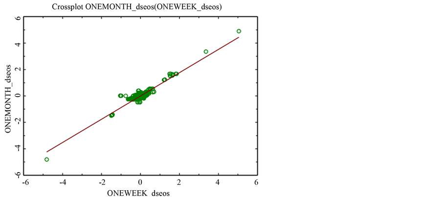
Figure 3. Euribor in level Nadaraya-Watson regression (one week versus one month).
the Optimization Toolbox of the MATLAB Software to locate the minimum of the negative log-likelihood function. The routine implements a subspace trust region method which is based on the interior-reflective Newton method described in [29] and [30] . Each iteration in this “large-scale optimization” algorithm involves the approximate solution of a large linear system using the method of reconditioned conjugate gradients. The principle of maximum likelihood estimation (MLE), originally developed by R. A. Fisher in the 1920s, states that the desired probability distribution be the one that makes the observed data most likely, which is obtained by seeking the value of the parameter vector that maximizes the likelihood function L(Z). The vector of parameter estimated in each maturity can be written as:

To compare different processes for different maturities of the ECB interest rate, we estimate two nested models on the data set. We start estimating the combining expression of the Poisson-Gaussian model of Equation (11), then we treat apart the Gaussian model of a pure Gaussian model .
.
Table 5 and Table 6 present respectively the estimation of Poisson-Gaussian and pure Gaussian processes on daily data. The total number of observation is 2150. Estimation is carried out using maximum-likelihood incorporating the transition density seen previously in Equation (12).
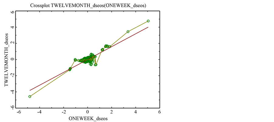
Figure 4. Euribor in first difference Nadaraya-Watson regression (one week versus twelve months).
Table 5. Basic Poisson-Gaussian estimation.
Bollerslev and Wooldridge (1992) robust t-statistics are in parentheses [31] .
Table 6. Basic Pure Gaussian estimation.
Bollerslev and Wooldridge (1992) robust t-statistics are in parentheses [31] .
Intuitive results emanate from this analysis. There is no evidence of skewness , but kurtosis exists
 . The jumps tend to be of the order of (3.17) basis points for shorter interest rate maturities and (2.55) basis points for a considerable one.
The jump intensity or the ex-ante probability of a jump occurring is better seen in a Poisson-Gaussian model than in a pure Gauss model because it encompasses maximum number of parameter estimated.
Figure 5 explores results of Gaussian-Poisson model estimation for different maturities. The shape of the likelihood function is shown in Figure 6. First difference of kernel density tells us the likelihood (“unnormalized probability”) of a particular parameter value for a fixed data set.

Figure 6. Probability Plots (first derivative of kernel density).
Note that the likelihood function takes the form of a curve if there is only one parameter beside h; which is assumed to be known. For example, if the model has two parameters, the likelihood function will be a surface sitting above the parameter space. In general, for a model with k Parameters, the likelihood function takes the shape of a k-dim geometrical “surface” sitting above a k-dim hyperplane spanned by the parameter vector.
The unconditional probability density function from the raw data and the plots from the best fitted models of each maturity is presented3. The upper panel plots the full distribution over the range 3 × 10⁻². The middle panel presents the same distribution but for a bigger value of h which is equal to 0.5, the closer plot clearly brings out the good fit from the ARCH-jump model compared to the other models. The lower panel deals with a representation from first derivative of kernel density which deviates negatively from the origin axe.
4.2. Day of the Week Effect Recognition
In this section, we shall employ the model to examine various phenomena in the bond markets via the lens of the model. Our jump model is facile in permitting many different analyses. We explore whether fluctuations are more likely to happen in predetermined days only for five operative days of the week (Monday, Tuesday, Wednesday, Thursday, and Friday). Our purpose is to determine which day is the favourable for announcing a supervising decision that can affect the market.
It is well known that fluctuations would be more likely on Monday since the release of non observable information over the weekend may lead to a larger volatility of the interest rate. Moreover, option expiry may inject fluctuations into the behaviour of interest rate on Wednesday and Thursday.
We focus our analysis on the last day of the operative week for the ECB and we determine the contribution of the other days in amplifying the arrival intensity of jumps in that day.
To be more precise, let illustrate what we had said before in a simple linear model that enable us to take into consideration the arrival intensity of fluctuation (rise or full) in the interest rate for different maturities:
 (25)
(25)
where , t = 1,2,3,4,5,6 is the temporal jump component, respectively for one week, one month, three months, six months, nine months and twelve months.
  is the arrival probability of a fluctuation if the chosen day is Friday, and
  is the incremental arrival intensity of jumps over Friday’s level when the day of the week take the possible day
 .
.
The following Table 7 presents results of the estimation of a jump-diffusion model when the jump arrival intensity is assumed to be influenced by the day of the week explored in the previous equation.
5. Concluding Remarks
We treat in this paper the evolution of the daily euro interbank offered rate to describe the announcement channel of the European Central Bank. The latter is computed daily for interbank deposits with a maturity of one week, one month, three months, six months, nine months and twelve months.
To provide a tutorial exposition of the maximum likelihood estimation, we evaluate results from basic Gaussian and Poisson-Gaussian models and try to compare the eventual illustrative results adopting these processes. Moreover, we conclude that jumps are an essential component for modeling EURIBOR. The illustrative Poisson and Gauss processes implemented in a linear model contribute to a much better in-sample fit once jumps are considered under either one or two models. We conclude that models do not lead to the same conclusions. It is the Poisson-Gaussian model that gives better performance. Searching for the contribution of day of the week in amplifying operative actions in the announcement channel of the ECB that consolidates the link with the market, we have resorted to a third linear model deeply linked to the previous parameter estimated through a Poisson
Table 7. Jump estimation parameter with day of the week effects.
Bollerslev and Wooldridge (1992) robust t-statistics are in parentheses [31] .

Figure 7. Mondays effect (estimation with , maturity = one month).

Figure 8. Wednesdays pertinent effect (estimation with , maturity = one month).
Gaussian model. Therefore, we have added dummy variables to conclude after estimation that only Mondays and Wednesdays for each maturity taken and especially for one month can represent the preponderant days that contribute to amplifying the jumps that may occur on Fridays (Figure 7 and Figure 8 ). The maintenance period effect and the calendar effect cause greater jumps than the effect of the meetings of the Governing Council of the ECB. The lowest jump intensity corresponding to the days on which none of the effects occur leads to the conclusion that when the ECB initially started to implement the single monetary policy, it faced a whole string of specific uncertainties ([24] [25] ). One such uncertainty concerned the way in which the transmission mechanism would function especially when that concerns the annoucement channel. The Poisson-Gaussian distribution was an attractive choice as a mixing distribution for models of Euribor data that exhibit over dispersion caused by the hierarchical structure. But it is also interesting to know in a further research whether gamma distribution can be applied to analyzing data for ECB.
NOTES
*Corresponding author.

1Cited from www.euribor.org, status at June, 10th 2006. For the complete list of panel banks, see www.euribor.org\html\content\panelbanks.html

2Inflation was admittedly still high despite the fall in oil prices and was picking up again in March-April. This can be explained as the result of the mad cow disease, i.e. an external supply shock.

3See Appendix for results of kernel density estimation (Table A1).