1. Introduction
Since Dantzig invented the simplex method [1] , the Linear Programming (PL) has been applied to solving problems from many research areas. In 1984 Karmarkar presented interior point algorithm for solving linear programming [2] without the inconvenience of the exponential complexity of the Simplex algorithm.
The article [3] presents an application of linear programming in power system engineering concerning system operation issues, like generation scheduling, loss minimization and also economics aspects such as planning of capital investments in generation equipments. It was presented a review of the linear programming utilization as well as some extensions to the techniques like the integer and quadratic programming and analyzed the incorporation of financial aspects to the problem. In [4] it is possible to see an application of linear programming in the determination of coordinated relay settings through a two-phase simplex method. Another application of linear programming is presented in [5] and reference [6] was pointed out the utilization of linear programming as one of the techniques to solve the unit commitment problem.
Proportional-Integral-Derivative (PID) controllers are a very efficient solution to obtain the desired output from the plant in steady state as well for dynamic response. Due to this aspect, the utilization of PID controllers has become very popular. The references [7] [8] present the main tuning methods utilized in academic research as well in industry. Two classical methods that are still utilized are the Ziegler-Nichols and the Cohen-Coon which utilize analytical approaches for analysis and tuning.
There are other analytical methods as described in [9] . Usually these methods employ heuristics [10] or intelligent methods like genetic algorithms [11] , differential evolution [12] and particle swarm optimization [13] . These approaches demand the existence of a population according to an evolution criterion. Although these methods present good results, usually the computational time is high and requires several parameters tunings. One advantage of these methods is the fact that the objective function can be a heuristic rule that weights the output signal in various aspects at the same time.
However, despite of the fact that this characteristic is an advantage, the complexity of the objective function and the number of restrictions of the system increase the nonlinearity and the probability of the system is no convex. This characteristic can lead the population based optimization methods to have convergence problems [14] [15] .
Seeking a faster and more efficient methodology for PID controller, this paper presents the development of a novel technique to tune the proportional-integral and derivative gains. As stated before, this device has been widely used as shown in many works encouraging the investigation of the possible improvements when it is tuned by using Linear Program (PL) based on interior point optimization, well known in several areas [16] [17] but still unexplored in the proposed area.
The main advantage of the proposed method resides on the fact that the systems designer can define the desired output in order to avoid saturations or other features and the optimization algorithm will return the appropriate PID parameters values that minimize the error between the actual and the desired output. Manipulating the system to isolate the PID terms results in a linear optimization problem, with convex space solution, restricted and rapidly solved with the interior point optimization method.
This article is organized in the following manner: in Section 2 basic concepts of PID tuning are described; in Section 3 the methodologies employed are presented; in Section 4 the system model is shown and a detailed tutorial example is presented to illustrate the methodology. At the end of Section 5 the results with an autonomous submarine are presented and in Section 6 some conclusions are presented.
2. Basic Concepts
The standard system model considers the Plant G(s) and PID Controller structure as showed in Figure 1. In this figure C(s) represents the output response of the plant assuming a generic input R(s). The PID controller is composed by three terms whose transfer function is given by:
 (1)
(1)
where PIDaction and PIDin represent respectively the output and input signals of the PID controller. The parameters Kp, Ki and Kd are, respectively the proportional, integral and derivative gains. The time constant Td represents the derivative filters parameter to reduce a high frequency noise. In practices Td = kd leading in this work to adopt Td equal to 0.001.
Roughly speaking, the Kp term provides a proportional action to the input signal PIDin, the Ki term eliminate the steady state error and the Kd term reduce the transitory oscillations.
Therefore when the controller gains are correctly tuned, the associated PID controller can provide good results with linear and nonlinear systems considering small parameter variation. The dynamical and steady state performance requirements can be achieved through the specification of some criteria in time and frequency domain, for example, the minimization of the quadratic error.
3. Proposed Methodology
For the application of the proposed methodology, the standard representation of Figure 1 should be redrawn as shown in Figure 2 where the proportional and integral controllers were combined in a single block. In this diagram the signal (PIaux) represents the output of the proportional-integral block, (Dv) and (Daux) the output of the derivative one. It is easy to verify that the output of the PID block (PIDout) is the sum of all control actions.
Considering that the output of the plant CS(t) is pre-specified by the designer face to a disturbance R(t) and using numerical integration method as described in Appendix, it is possible to determine the PIDin(t) signal. It can be seen from Figure 2 that PIDout(t) is equal to CS(t). So the problem is to determine the parameters of the PID blocks to match the input PIDin(t) and output PIDout(t) signals.
Equations (2)-(4) describe the PID formulation in terms of parameters Kp, Ki, Kd and input/output signals showed in Figure 2:
 (2)
(2)
 (3)
(3)
 (4)
(4)
Comparing PI block with generic transfer function given in Appendix, it is possible to obtain:
 (5)
(5)
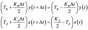
Then the values of parameters gamma defined in Equations (A.8) are:
 (6)
(6)
Therefore Equation (A.7) can be rewritten as follows:
 (7)
(7)
where . Considering Equations (3) into Equation (7) yields to:
 (8)
(8)
Rearranging (8), leading to Equation (9), as follows:
 (9)
(9)
where:
 (10)
(10)
 (11)
(11)
After obtaining all vectors of Equation (9), it is possible to calculate the parameters Kd,  and
and  by using the linear programming formulation to take adjustable input and output signals. In this way, the optimization problem can be formulated as shown in Equations (12):
 (12)
(12)
where Te: Total error of the fitting from linear programming;
N: Number of equality constraints that is equal to the C(k) length;
R1: Vector of right positive residue in the RN subspace;
R2: Vector of left positive residue in the RN subspace;
ub: Upper bound of residue variables. The ub equal to 200 is adopted in this paper. The rangers adopted for other variables have been enough to find the desire fitting.
Hence, considering an input and output signals with N values, it is possible to obtain a set of N-1 equations given by Equations (9) which is the set of constraints of the optimization problem (12). Nonetheless it is numerically unlikely that the equality constraints imposed by Equation (9) can be completely satisfied, thus the positive residue variables R1(k) and R2(k) is added to provide enough slacks in the constraints. Then, the objective is to minimize the sum of these residues.
The compact form of problem (12) is written according to a linear optimization problem:
 (13)
(13)
where:

and  a vector with all elements equal to one.
Thus:

The proposed LP problem (12) has spent low computational time because it has been written as a linear program and solved by using the ToolBox called linprog of MATLAB© based on a linear interior point solver [18] , which is a variant of the Mehrotra’s predictor-corrector algorithm [19] . The advantage of using linear programming is related to a convex region close to a viable operating point. So, even under about one thousand linear constraints, the problem (12) spends about 3 seconds to find the solution.
Therefore, the solution of the LP problem (12) brings the values of the parameters Kd, ρ1 and ρ2 that better fit the input/output signals to minimize R1(k) and R2(k). By replacing Kd, ρ1 and ρ2 in the set of Equation (6), it is possible to calculate the values of Kp and Ki
4. Results
The results of the application of the proposed methodology will be presented in two parts, the first one dedicated to a tutorial case and the second one to tuning of an attitude control for vertical orientation of a vehicle in launching stage.
The time to complete the whole optimization process was only 3 sec in a MacBook pro core i5 with 4 Gb of RAM and the algorithm implemented in MATLAB© script program.
4.1. Tutorial Analysis
For this tutorial analysis it was chosen the plant from Equation (14) represented by its transfer function G(s) as described in reference [20] .
 (14)
(14)
The specified output CS(t) in response to a unit step input R(t) can be seen in Figure 3. This curve was obtained by using a standard second order model given by:
 (15)
(15)
With ωn = 3, ζ = 1, Δt = 0.01 and time simulation equal to 7 seconds. It can be emphasize that the total elements of vector CS(t) is equal to N = 7/0.01 = 700 points.
Considering the model presented in Figure 2, it is necessary to obtain all points of the curves utilized as coefficients in the composition of the optimization problem (12). Therefore, with a unit step R(t) and the specified Cs(t), the input signal E(t) to the plant transfer function G(s) is given by E(t) = R(t) − CS(t) whose curve is shown in Figure 4.
Figure 5 shows the input signal of PID controller (PIDin) that is obtained from E(t) as input signal of G(s) and using trapezoidal integration showed in Appendix.
The last set of points needed to complete the coefficients of the problem (12) is Dv(t) obtained from PIDin by using Equation (4) and trapezoidal integration. Figure 6 displays Dv(t) signal.
After all coefficients were calculated, it is possible to build the optimization problem (12) for the optimal PID parameter calculation. Using the LP Toolbox of Matlab Kd, ρ1 and ρ2 are obtained to match the input and output signals with the total error of the fitting (Te) equal to 0.037. From Equations (6), it is possible to calculate the values of Kp and Ki. Table 1 shows the best values of PID parameters obtained by the optimization process. In addition, the second row of the table shows the PID proposed in reference [20] .
To evaluate the performance of the proposed methodology a simulation using the system of Figure 1 were carried out for both adjustable PID calculated from LP and PID of the literature [20] . Figure 7 presents these output results including CS(t). It can be observed that the methodology based on LP resulted in a best behavior compared with literature. In addition, this figure shows that the C(t) followed the specified output being practically identical to the desired one.
Figure 8 presents the initial PIDaction related with the peak signal. This feature is important to avoid the action control reaches the saturation limit. As seen in Figure 8, the maximum peak signal in the proposed LP approach is much lower than the corresponding peak displayed in literature [20] . Although it is not in the scope of this work, it is possible to modify the CS(t) in order to find other initial PIDaction.
4.2. Attitude Control
A basic flight of vehicle is composed by guidance, navigation and an attitude control systems [21] . The last one control system is responsible for vehicle vertical orientation. Usually, the utilization of conventional controller tuning techniques presents unsatisfactory performance due to plant characteristics. The proposed methodology will be applied to the PID design for the attitude control, in particular to maintain the vertical angle in respect with the vertical in 0˚. Thus this problem is similar to the control angle problem of the Inverted Pendulum Model (IPM).
The linearized equation that represents the rotation movement of the shaft in respect with the center of gravity can be defined by:
 (16)
(16)
where θ is the relative shaft angle in respect with the vertical axe; l is the length of the shaft; M is the mass of the mobile support and is equal to 2 kg; m is the shaft mass and is equal to 0.1 kg; g is the acceleration of gravity, considered 9.81 m/s2; u represents the force produced by the PID control effort.
Applying the Laplace transform and replacing the numerical values it is possible to obtain the simplified

Table 1. The PID controller parameters.
model in frequency domain resulting in Equation (17). In a preliminary analysis it is possible to note that the resulting model is difficult to control due to the positive real part of one of the poles.
 (17)
(17)
In this case, since it is an inverted pendulum model (IPM), the system response must be fast and stable. Thus, the specified output signal CS(t) necessary to train the system is defined by the following parameter values ωn = 50, ξ = 1 and 0.25 seconds of training time with an integration step of Δt = 0.001. Considering an impulse of 0.01 rd (0.573˚) to stimulate the system and replacing these values in Equation (15), it can be obtained the curve
showed in Figure 9. In this case, the total elements of vector CS(t) is equal to N = 0.25/0.001 = 250 points. This is the considerable amount of points in order to successfully complete the optimization process.
As seen in Figure 9, it must have a reduced time simulation for training control action to avoid the pendulum falls. Although there are strategies to automatically deal with this problem, it is out of the scope of this work. Therefore, the time simulation for training output signals is considered provided heuristically by the designer experience.
In Table 2 it is shown the both PID gain values by the proposed methodology and reference [20] for the inverted pendulum model of the attitude control problem.
The performance of the proposed PID tuning is evaluated by using the system of Figure 1 where the time simulation of 2 sec was adopted. Figure 10 shows the output simulations of C(t) for proposed, literature and specified. It can be observed that the LP approach presented the best behavior because the initial angle varies less than the PID adjusted from literature. It is important to mention that this feature results in less chance of the pendulum falling to or the control strategy just fails. In addition, the figure shows that the proposed PID tuning is capable to follow the specified output.
Figure 11 presents the initial PIDaction related with the peak signal. This feature is important to avoid the action control reaches the saturation limit. As it was expected the proposed PID tuning has resulted in a slower peak response with a smaller overshoot due to the derivative block.
Table 2. PID attitude control parameters.
Analyzing the obtained results it is possible to observe that the optimized performance of the proposed controller was able to maintain the desired angular position for the projectile.
5. Conclusions
This article presented a method based on linear programming for the tuning of PID controller parameters using a primal-dual interior point method. From the known system plant model and a specified desired output signal, it is possible to use generic transfer functions to isolate the PID parameters as the only unknown system variables. This transformation allows the formulation of a linear optimization problem that can be solved with small computational effort with satisfactory results.
The method was described with the aid of a detailed tutorial analysis and a specific case of the attitude control of a flight vehicle was also analyzed obtaining excellent results. From the results obtained applying the proposed methodology the following aspects can be stressed out:
• The specified plant output can always be obtained close to the desired one with negligible error, if the system dynamics and saturation are considered.
• The obtained optimization problem is linear presenting a convex feasible region resulting in numerical robustness.
• The computational time is small even with a large quantity of sample points for the training process.
• The proposed method can be modified to use nonlinear plant models once the curve construction processes are made outside the optimization stage.
• An extension of the methodology can be applied to adaptive control considering that the computational time is compatible with data acquisition time of the variables.
Acknowledgements
The authors would like to thank FAPEMIG, CAPES/PNPD and CNPq for the financial support.
Appendix: Transfer Function Solution
This appendix presents the steps for the numerical integration process based on trapezoidal method. Therefore, a solution to a generic transfer function is presented in Equation (A.1) which is possible to represent a wide range of linear models for real plants. In this equation, X(s) represents the input signal and Y(s) is the output.
 (A.1)
(A.1)
Manipulating (A.1) and rearrange one yield:
 (A.2)
(A.2)
In time domain Equation (A.2) becomes:
 (A.3)
(A.3)
or
 (A.4)
(A.4)
Integrating both sides of (A.4) it is possible to obtain:
 (A.5)
(A.5)
Solving Equation (A.5) by using the trapezoidal integration method, leads to:
 (A.6)
(A.6)
Simplifying Equation (A.6), it results:
 (A.7)
(A.7)
where:
 (A.8)
(A.8)
It can be observed that Δt represents the step of the numerical integration. In addition, it is important to emphasized that the output signal y(t) can be obtained from input signal x(t) and parameters block ( and
and ). On the other hand, if both input x(t) and output y(t) are known it will be possible to obtain the parameters
 ,
,  and
and . This issue will be solved in the proposed methodology by using Linear Programing (PL) approach. In all cases, both vectors x(t) and y(t) have the same number of elements (N). For example, for time simulation equal to T = 10 seconds and Δt = 0.01, the vectors x(t) and y(t) will have T/Δt points corresponding to one thousand elements.