The Luminosity Function of Galaxies as Modeled by a Left Truncated Beta Distribution ()
1. Introduction
The standard luminosity function for galaxies (LF) in the last forty years has been represented by the Schechter LF
 (1)
(1)
where  sets the slope for low values of
 ,
,  is the characteristic luminosity and
  is the normalization, see [1] . This LF is defined in the in the interval
  and has replaced other LFs presented by [2] -[5] .
The goodness of the fit can be evaluated by the merit function 
 (2)
(2)
where n is number of data and the two indexes  and
and  stand for theoretical and astronomical, LF respectively. The value of
  which characterizes the Schechter LF for a given astronomical catalog, i.e. the Sloan Digital Sky Survey (SDSS) in five different bands, represents a standard value to improve. Many new LFs has been derived in the last years and we report some examples. A two-component Schechter-like function is, see [6]
 (3)
(3)
where

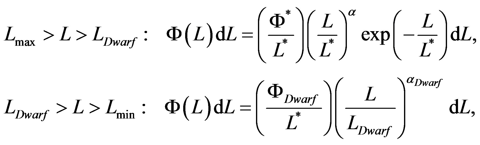
This two-component LF defined between the maximum luminosity,  , and the minimum luminosity,
  , has five parameters because two additional parameters have been added:
  which represents the magnitude where dwarfs first dominate over giants and
  which regulates the faint slope parameter for the dwarf population.
In order to fit the case of extremely low luminosity galaxies a double Schechter LF with five parameters, see [7] , was introduced:
 (4)
(4)
where the parameters  and
and  which characterize the Schechter LF have been doubled in
  and
and . The strong dependence of LF on different environments such as voids, superclusters and supercluster cores was analyzed by [8] with
 (5)
(5)
where  is the exponent at low luminosities
 ,
,  is the exponent at high luminosities
 ,
,  is a parameter of transition between the two power laws, and
  is the characteristic luminosity. Another LF starts from the probability density function (PDF) that models area and volumes of the Voronoi Diagrams and introduces the mass-luminosity relationship, see [9] ; in the SDSS case
 . A last example is represented by three new LFs deduced in the framework of generalized gamma PDF, see [10] ; in the SDSS case
 . All the previous LFs cover the range
  and therefore the analysis of finite upper and lower boundaries can be a subject of investigation. Another interesting observational fact is that at low values of luminosity (high absolute magnitude) the observed LF has an approximate constant value. The left truncated beta with scale PDF recently derived , see Equation (34) in [11] , satisfies the two issues previously raised. In order to explore the connection between LF and evolution of galaxies see [12] -[18] .
Here we analyze in Section 2 a left truncated beta LF for galaxies and in Section 3 a left truncated beta for mass which transforms itself in a LF for galaxies through a nonlinear mass-luminosity relationship. Section 4 reports a recent LF for galaxies which has a finite boundary at the bright end.
2. A Linear Mass-Luminosity Relationship
A new PDF, the left truncated beta with scale has been recently derived, see formula (34) in [11] . Once the random variable X is substituted with the luminosity L we obtain a new LF for galaxies,  ,
,
 (6)
(6)
where  is a normalization factor which defines the overall density of galaxies, a number per cubic Mpc. The constant
  is
is
 (7)
(7)
and ,
,  are the lower, upper values in luminosity and
  is the regularized hypergeometric function [19] -[23] . The hypergeometric function with real arguments is implemented in the FORTRAN subroutine MHYGFX in [24] . The averaged luminosity,
  , is:
, is:
 (8)
(8)
where

The relationships connecting the absolute magnitude M,  and
and  of a galaxy to respective luminosities are:
 (9)
(9)
where  is the absolute magnitude of the sun in the considered band. The LF in magnitude is
 (10)
(10)
where
 (11)
(11)
This data-oriented LF contains the five parameters ,
,  ,
,  ,
,  ,
,  which can be derived from the operation of fitting the observational data and
  which characterize the considered band. The number of variables can be reduced to three once
  and
and  are identified with the maximum and the minimum absolute magnitude of the considered sample. The numerical analysis points toward value of
 . Once as an example we fix
  we have only to find the two parameters
  and
and . The test on the new LF were performed on the data of the Sloan Digital Sky Survey (SDSS) which has five bands u*, g*, r*, i*, and z*, see [25] . Table 1 reports the bolometric magnitude, the numerical values obtained for the new LF , the number, N, of the astronomical sample , the
  of the new LF, the reduced
 ,
,  , of the new LF, the
  of the Schechter LF, the reduced
 ,
,  , of Schechter LF and the
  computed as in [25] for the five bands here considered.
3. A Non Linear Mass-Luminosity Relationship
We assume that the mass of the galaxies,  , is distributed with a left truncated PDF as represented by formula (34) in [11] . The distribution for the mass is
  where
where  is the lower mass and
  is the upper mass. The mass is supposed to scale as
 (12)
(12)
where c is the parameter that regulates the non linear mass-luminosity relationship. The differential of the mass is
 (13)
(13)
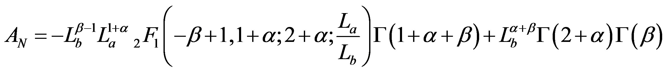
As a consequence the LF representing the non linear mass-luminosity relationship is
 (14)
(14)
where
 (15)
(15)
The averaged luminosity,  , for the non linear mass-luminosity relationship is:

Table 1. Parameters of fits in SDSS Galaxies of LF as represented by formula (10) in which the number of free parameters is 5.
 (16)
(16)
where

The LF in magnitude for the non linear mass-luminosity relationship is
 (17)
(17)
where
 (18)
(18)
Table 2 reports the numerical values obtained for the new nonlinear LF as represented by Equation (17), the  of the new LF and the
  of the new LF in the five bands here considered.
The Schechter LF, the new LF represented by formula (17) and the data of SDSS are reported in Figure 1-5, where bands u*, g*, r*, i*, and z* are considered.
A discussion on the distribution of M/L in all photometric bands can be found in [26] .
4. A Modified Schechter LF
An example of modified Schechter LF is represented by the following function
Table 2. Parameters of fits in SDSS Galaxies of LF as represented by our non linear LF (17) formula (10) in which the number of free parameters is 6.
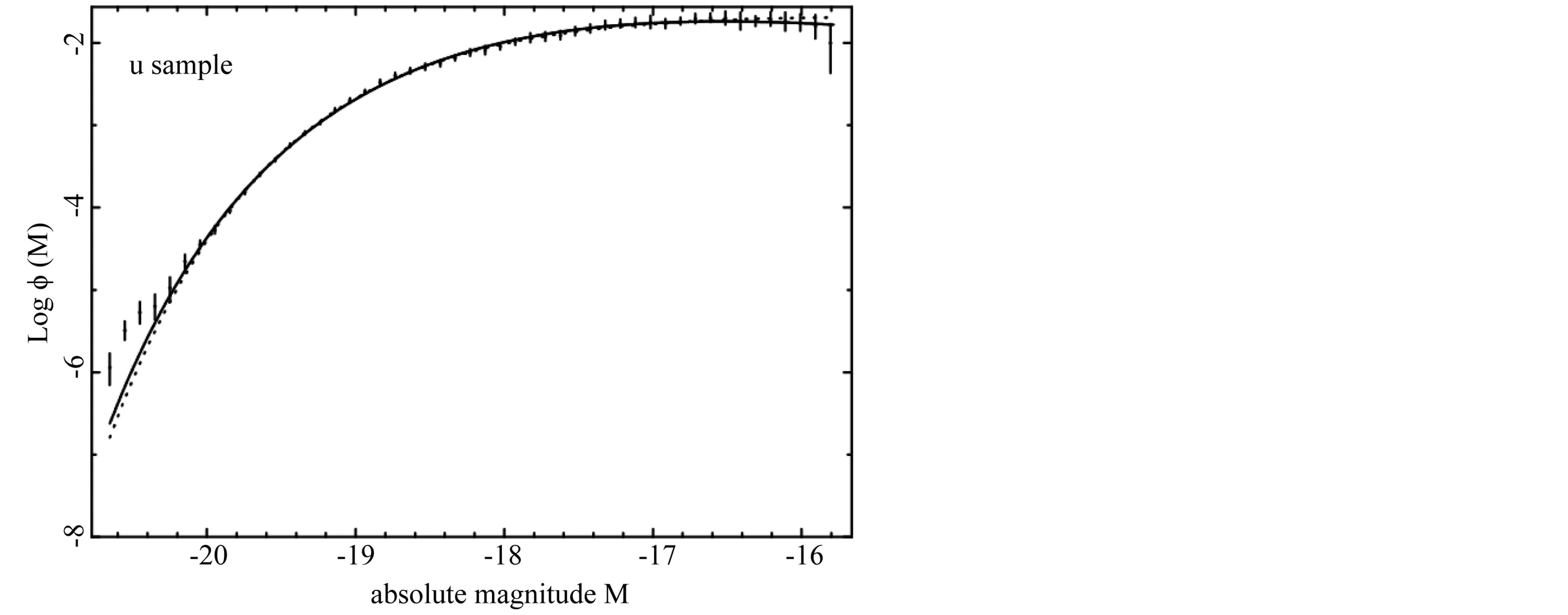
Figure 1. The LF data of SDSS (u*) are represented with error bars. The continuous line fit represents our non linear LF (17) and the dotted line represents the Schechter LF.

Figure 2. The luminosity function data of SDSS (g*) are represented with error bars. The continuous line fit represents our non linear LF (10) and the dotted line represents the Schechter LF.

Figure 3. The luminosity function data of SDSS (r*) are represented with error bars. The continuous line fit represents our non linear LF (10) and the dotted line represents the Schechter LF.
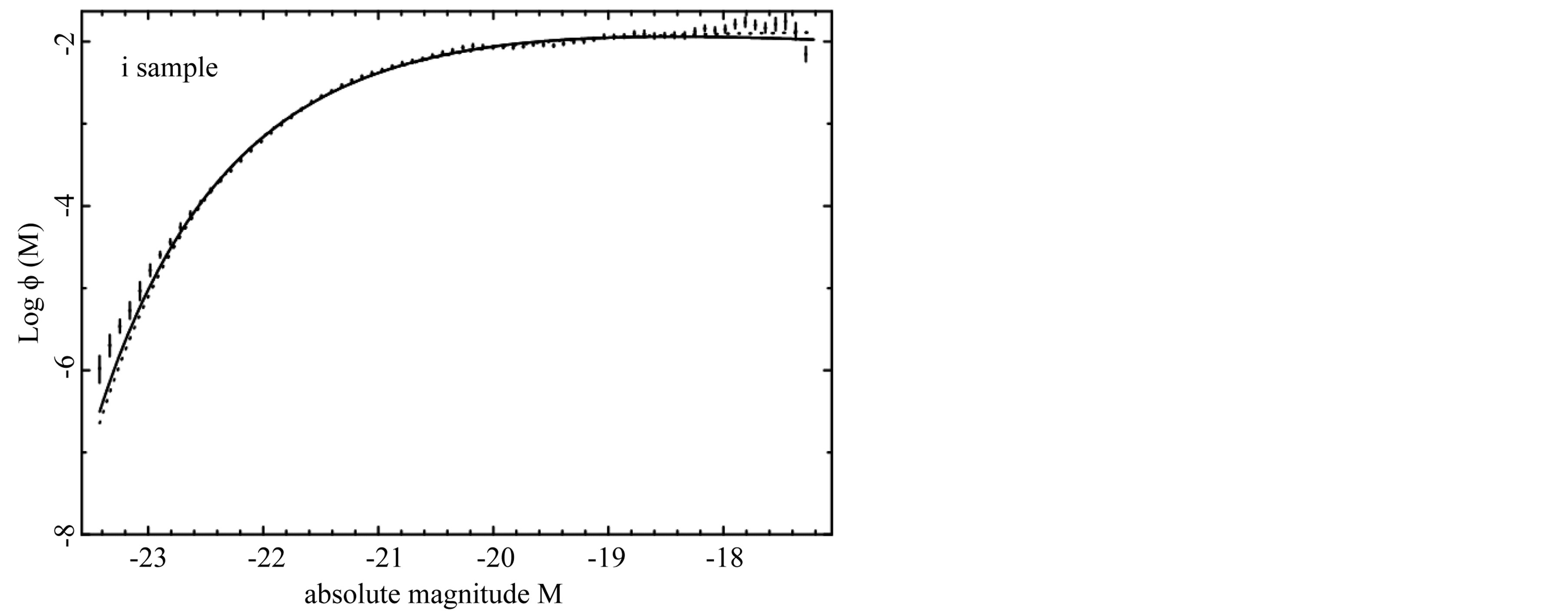
Figure 4. The luminosity function data of SDSS(i*) are represented with error bars. The continuous line fit represents our non linear LF (10) and the dotted line represents the Schechter LF.
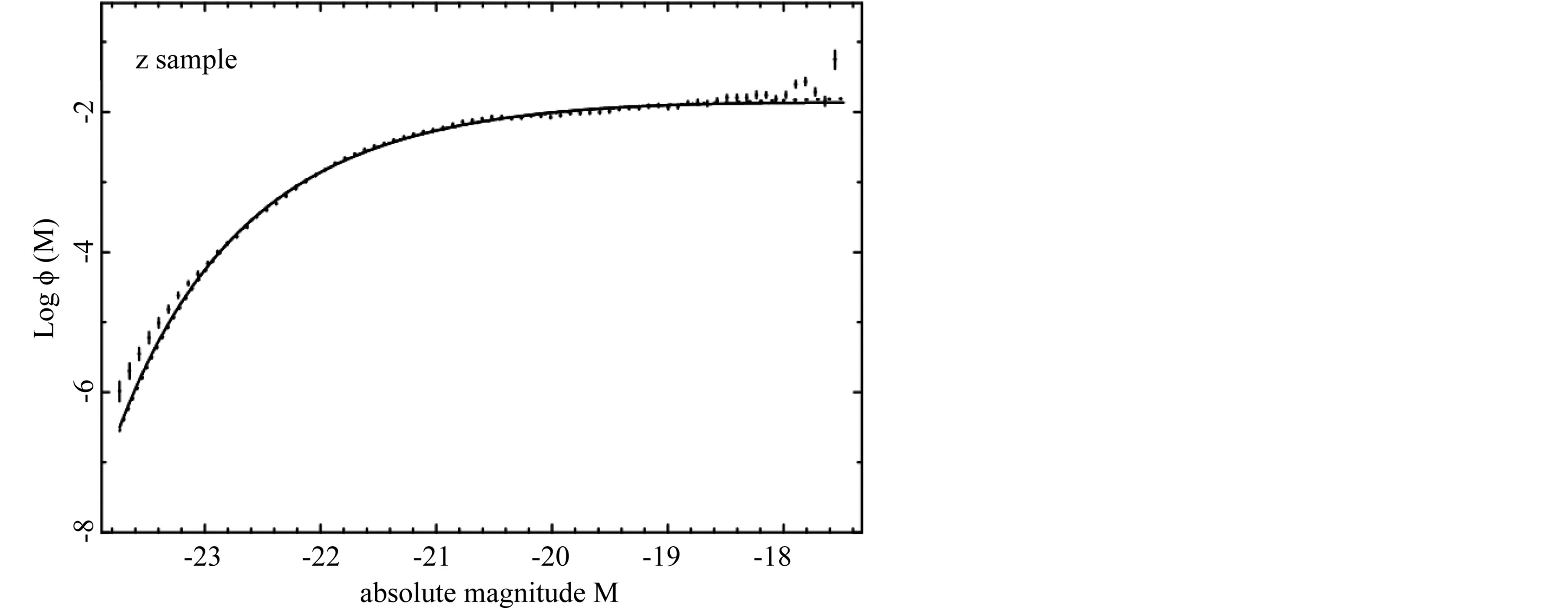
Figure 5. The luminosity function data of SDSS(z*) are represented with error bars. The continuous line fit represents our non linear LF (10) and the dotted line represents the Schechter LF.
 (19)
(19)
where  is a new parameter, see [27] . This new LF in the case of
  is defined in the range
where  and therefore has a natural upper boundary which is not infinity. In the limit
 the Schechter LF is obtained. In the case of
  the average value is
 (20)
(20)
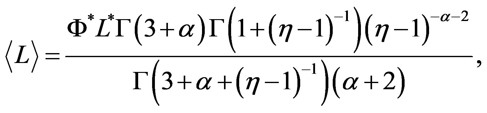
and in the case of  the average value is
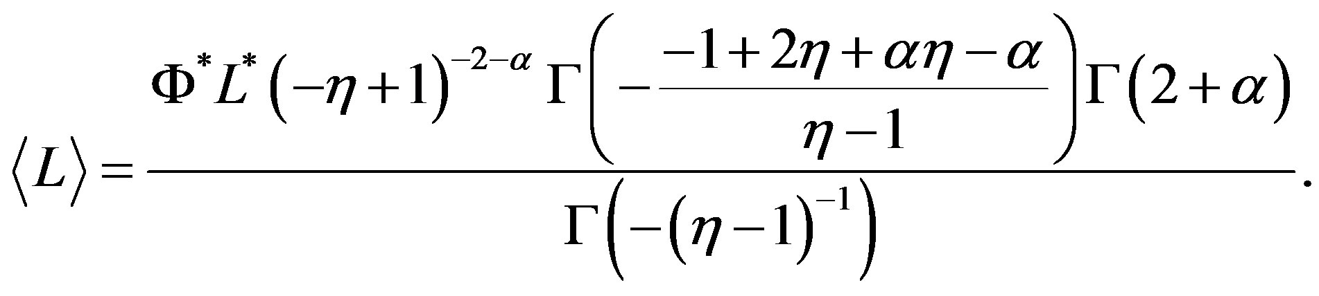 (21)
(21)
The distribution in magnitude is:
 (22)
(22)
As an example the Schechter LF, the modified Schechter LF represented by formula (22) and the data of SDSS are reported in Figure 6 for the u* band and Table 3 reports the results of the fits in all the five bands of SDSS.
5. Conclusions
Motivations The observational fact that the LF for galaxies spans from a minimum to a maximum value in
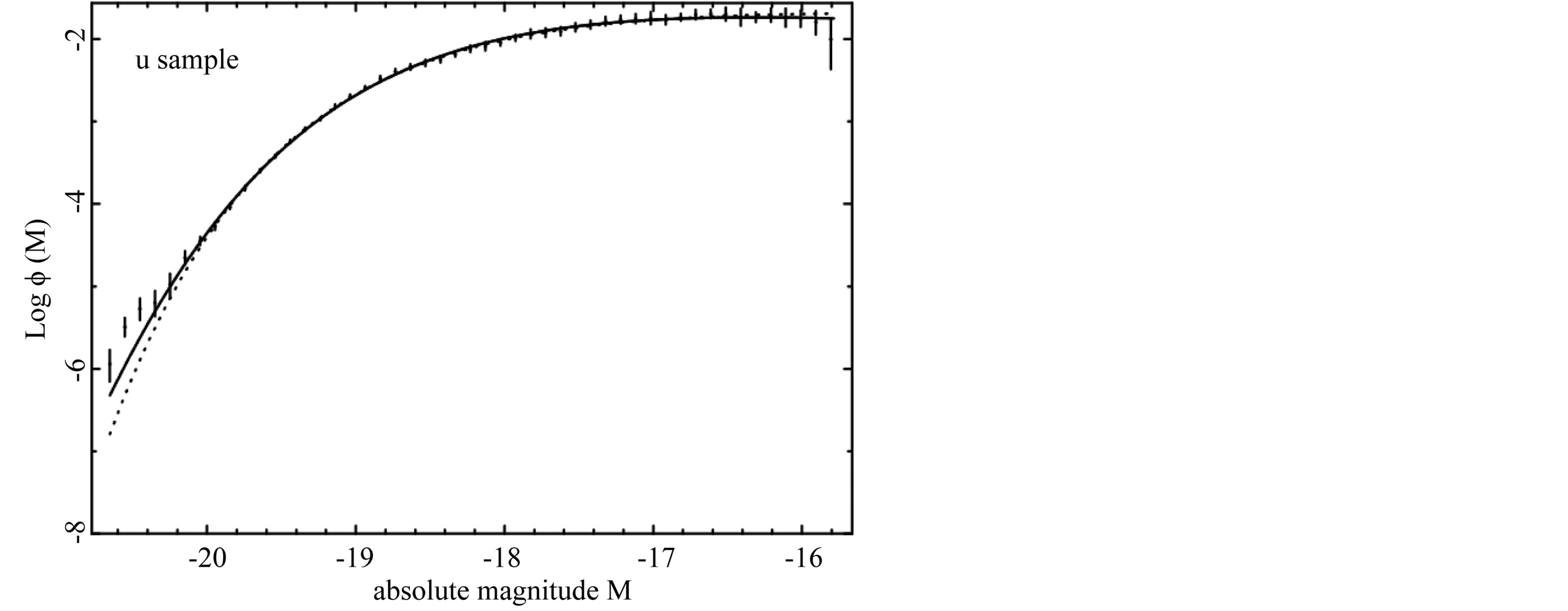
Figure 6. The luminosity function data of SDSS (u*) are represented with error bars. The continuous line fit represents the modified Schechter LF (22) and the dotted line represents the Schechter LF.
Table 3. Parameters of fits in SDSS Galaxies of the modified Schechter LF as represented by formula (22) in which the number of free parameters is 4.
absolute magnitude makes attractive the exploration of the left truncated beta LF. We derived two LFs adopting the framework of the linear M-L relationship, see Equation (10), and the framework of the non linear M-L relationship , see Equation (17).
5.1. Goodness of Fit Tests
We have computed  and
and  for two LFs here derived and compared the results with the Schechter LF, see Tables 1 and 2. In the linear M-L case
  and
and  are greater of that of the Schechter LF. In the non linear M-L case
  and
and ,
,  and
and  , are smaller in two bands over five in respect to those of the Schechter LF. The non linear case suggests a power law behavior with an exponent
  and therefore M-L relationship has an exponent greater than 1 but smaller than 4 , the theoretical value of the stars.
5.2. Modified Schechter LF
The modified Schechter LF when  , which is the case of SDSS , has by definition an upper boundary, see 4. The
  and
and  are smaller in five bands over five in respect to those of the Schechter LF. This goodness of fit is due to the flexibility introduced by the fourth parameter
  as outlined in [27] .
5.3. Physical Motivations
The Schechter LF is motivated by the Press-Schechter formalism on the self-similar gravitational condensation. Here conversely we limited ourself to fix a lower and an upper bound on the mass of a galaxy and we translated this requirement in a PDF for mass and then in LF. Finite-size effects on the luminosity of SDSS galaxies has also been explored in [28] .