The importance of household composition in epidemiological analyses of sleep: Evidence from the Understanding Society longitudinal panel survey ()
What this study adds: This research project demonstrates that household composition can be reliably operationalised using data on the age structure of household occupants and overcrowding to reveal the role that: the number of children in the household; large and extended families; and overcrowding play as predictors of sleep duration and sleep quality amongst adult household members.
Associations between sleep and cardiovascular disease, diabetes and mortality have been observed across a range of different studies and contexts [2]. However, fewer studies have documented the many contextual factors that predict or influence sleep, or the role of social structures, such as household composition, on sleep. Previous work examining which household characteristics might predict sleep has primarily considered relationships between the number of household occupants and either the number of children in the home or the ages of any children in the home [1-3]. Typical of these studies was that by Chapman et al. [1] who found that the frequency of “insufficient sleep” was highest in households with at least 3 children. However, most such studies have failed to fully explore the inter-relationships between these characteristics, and the role that broader sociodemographic patterns and housing structures might play as predictors of sleep.
Notable exceptions include Burgard et al. [4], who adopted a latent class analysis (LCA) approach to categorise study participants according to their “life course stage”. Their study, and that by Groeger et al. [3], suggested that factors such as partnership status and parental status have a significant association with sleep duration such that childless adults, for example, tend to have longer sleep durations compared than adults living with children. Neither of these studies (and none that we have been able to find) used LCA to consider overcrowding in the home as a potential predictor of sleep alongside the sociodemographic distribution of household occupants. Overcrowding is likely to have a substantial impact on sleep, and on the impact that partnership status, parental status and the number/ages of children in the household have on sleep.
To address this issue, the present study used data from Understanding Society (USoc), the United Kingdom’s nationally representative household panel survey, to: define household composition in terms of latent household classes; and examine the relationship between household composition and self-reported sleep duration and quality. The study aimed to extend our understanding of the household characteristics that are associated with sleep and thereby inform future epidemiological research, including the potential development of sleep interventions that are sensitive to variation in household composition.
2. METHODS
2.1. Study Participants
The first Wave of USoc [5] collected data from January 2009 to January 2011, and involved 50,994 participants from 30,169 households. The second Wave involved 54,597 participants from 30,508 households and took place from January 2010 to April 2012. Individual respondent data were collected from adults (16 years and over) using computer assisted personal interviews. Household data were collected from one adult member of each household acting as a key informant.
2.2. Household Composition Indicator Variables
The household variables used in the latent class analyses were the: number of adults; number of children; number of couples; number of single parents; number of pensioners; and an ordinal variable indicating the extent to which there was overcrowding in the home. This ordinal variable was created using the UK Government’s definition of household overcrowding, based on the “Bedroom Standard” measure within the “Household (Overcrowding) Bill” [6]. This involved calculating the ratio of the number of rooms used for sleeping (i.e. bedrooms) to the Bedroom Standard as a measure of overcrowding [6]. The Bedroom Standard was calculated using information provided by all household respondents on the total number of residents by age and sex in the household, a single bedroom being assigned for: each adult couple; any single adults aged 21 years and over; all pairs of same sex 10 - 20 year olds; and any pairs of children under 10 years of age, regardless of sex.
2.3. Sleep Variables
The present analyses drew on two sleep-related variables recorded during the first Wave of the study using the “Self Completion Adult Module” questionnaire. This collected self-reports of sleep duration (generating continuous data on hours of sleep) and sleep quality (generating categorical data based on “very good” to “very bad” sleep quality), based on two items in the questionnaire:
Sleep duration: “How many hours of actual sleep did you usually get at night during the last month? This may be different than the actual number of hours you spent in bed”.
Sleep quality: “During the past month, how would you rate your sleep quality overall?” Very good; Fairly good; Fairly bad; Very bad.
2.4. Descriptive Covariates, Confounders and Competing Exposures
Variables extracted from the Wave 1 USoc questionnaire to further characterize the latent household composition classes, and/or adjust for potential confounding in the polynomial logistic regression analyses of the relationship between household composition class and sleep duration/quality requiring adjustment, comprised: respondent age (calculated to the nearest year using self-reported date of birth and questionnaire completion date); respondent sex (as reported); the number of children aged 0 - 2, 3 - 4, 5 - 11 and 12 - 15 in the household; adult marital status (single, married/civil partnership, separated, divorced or widowed); highest educational qualification achieved (University degree+, post-school qualifications; A-level or equivalent; GCSE or equivalent, Other school qualification or none); ethnicity (White British, Other White background, Black, Black mixed race, Asian, Asian mixed race, or Other ethnic group); and SF12 single item self-rated health (Excellent, Very good, Good, Fair, Poor).
To establish which of the covariates might operate as potential confounders, mediators or competing exposures in the multinomial logistic regression analyses exploring the relationship between latent household composition class and sleep duration/quality, a causal path diagram was constructed in the form of a Directed Acyclic Graph (DAG), drawing on established and hypothesised functional relationships between the exposure variable (latent household composition class), the outcome variable (sleep duration/quality) and each covariate [7]. This DAG was uploaded to the freeware program DAGitty.net (see: www.dagitty.net; [8]) which uses established algorithms [9] to identify confounders (which cause both exposure and outcome), mediators (which are caused by the exposure and cause the outcome), and competing exposures (which are unrelated to the exposure but cause the outcome). DAGitty.net uses additional algorithms to identify any “minimum sufficient adjustment sets” (i.e. groups of available/measured covariates) that need to be included in any multivariable analyses to eliminate confounding (using “back-door paths”; [10]). The benefit of this approach is that it provides an explicit a priori model of the postulated relationships between the exposure and outcome variables and each of the available covariates. Such models are invaluable for the specification and subsequent verification of the statistical analyses, to ensure that these avoid the risk of over-adjustment or inappropriate adjustment for mediators (i.e. covariates that lie on the causal path between exposure and outcome; [11]). These models also help to establish whether the statistical models used are the most parsimonious (and therefore those with optimum statistical power) rather than simply (over)adjusting for all available covariates (with the resulting reduction in statistical power; [12]).
2.5. Latent Class Analysis (LCA)
Household manifest variables from both Waves 1 and 2 of USoc were analysed using latent class analysis (LCA) to define household composition as a latent categorical construct, using the sociodemographic variables and overcrowding index described earlier, and Latent Gold 4.5 software [13]. The manifest variables were treated as either indicator variables (i.e. dependent variables of the latent classes) or covariates (i.e. variables used to describe rather than measure or define the latent classes; [14]). Using an exploratory LCA approach, models were produced using indicators and covariates, each model defining the data based on a different number of latent classes. The Bayesian Information Criterion (BIC) was used to evaluate model fit and parsimony. The BIC provides a criterion for model selection amongst a group of models with differing numbers of parameters by taking into the account the sample size, the number of parameters included, and the maximized log-likelihood of each model [15]. The BIC also introduces a penalty term for the number of parameters in a model, and thereby accounts for over-fitting. The model with the lowest BIC value was therefore considered the best fitting model [16]. The best fitting models generated separately for data from Wave 1 and Wave 2 of USoc were then compared to assess the reliability and stability of latent household composition classes over time.
2.6. Multinomial Logistic Regression Analysis
Multinomial logistic regression analysis was undertaken on the Wave 1 data using Stata/IC 12.1 [17], to explore the relationship between latent household composition class membership and both sleep duration and sleep quality, after adjustment for any potential confounders and competing exposures identified using the DAG. These models generated measures of relative risk (RR) and their associated 95% confidence intervals (95%CI) which indicated the likelihood of experiencing any particular sleep outcome as compared to a referent sleep outcome for each of the latent household composition outcomes. For these analyses, self-reported sleep duration was categorized as: 5 hours or less; 5 - 6 hours; 6 - 7 hours; or 10 hours or more, and compared to a sleep duration of 7 - 8 hours as the referent. Self-reported sleep quality was categorized using the questionnaire item’s original answer categories as: “Very bad”; “Fairly bad”; or “Very good”, and compared to “Fairly good” sleep quality as the referent.
3. RESULTS AND DISCUSSION
3.1. Household Composition
Following an exploratory LCA of Wave 1 household manifest variables and covariates, a comparison of the BIC values for models with between 1 and 8 latent classes resulted in the selection of the model with 7 latent classes as the best-fitting model, based on the lowest log-likelihood BIC value of 267,652 (see Table 1). The labeling of each of the seven latent classes in the selected model, and the proportion and number of adult participants falling within each of these classes, has been summarized in Table 2. The labels developed to describe each of the seven latent household composition classes were based on the distribution of the manifest household variables, covariates and individual demographic characteristics, as detailed in Table 3.
The “Empty Nesters” class represents the largest latent household composition class (in which 51% of the total USoc sample were living), none of which had children living in the household, some of which comprise pensioners, but most of which comprise working-age adult couples. Members of this latent household composition class were all (100%) living in properties with more bedrooms than the Bedroom Standard and as such did not experience overcrowding.
The “Dwelling Sharing Childless Adults” class had fewer couples than the “Empty Nesters” and tended to represent adults living in smaller properties relative to the “Empty Nesters”, the majority (89.9%) having the same number of bedrooms as that prescribed by the Bedroom Standard.
The “Partnered with Child” and “Partnered with Children” classes were living in similar sized dwellings relative to household occupancy, the majority of these households (65.7% and 69.8%, respectively) having more bedrooms that the Bedroom Standard requirement.

Table 1. Latent class BIC model fit statistics.
However, these classes had different numbers of children, in that “Partnered with Child” had a mean of just 1.3 children in the household whereas “Partnered with Children” had at least one additional child (as reflected in the mean of 2.3 children).
In the “Large Family, Majority with Overcrowding’ class the majority of adults (mean = 2.231) were part of a couple with fewer single parents. This latent household composition class had the largest number of children of all classes (mean = 2.9), and the majority (63.2%) of these families were living in dwellings with fewer bedrooms than the Bedroom Standard requirement, the remainder (36.8%) living in homes that match the Bedroom Standard requirement.
The majority of adults living in the “Single Parent Household” class were single parents with a mean number of 1.4 children, and lived in properties that either met (61.5%) or had more bedrooms than (38.5%) the Bedroom Standard.
Finally, the “Extended Family, Majority with Overcrowding” class had the largest rate (at 76.5%) of overcrowding (i.e. the greatest proportion of households with fewer bedrooms than the bedroom standard) of all the latent household composition classes, and the largest number of adult occupants (mean = 2.630). The majority of adults were more likely to be part of a couple, less likely to be single parents and, on average, were living with 1 or more children (mean = 1.4).
To assess the reliability/temporal stability of the latent household composition classes identified from the analysis of data from Wave 1, these analyses were repeated with data from Wave 2 of USoc. Comparison of the BIC of models with between 1 and 8 latent classes demonstrated that a very similar model containing 7 similar latent classes was again the model of best fit with the lowest BIC of 268,362. Further similarities were evident from a comparison of the distribution of these classes, and of household manifest variables, covariates and indi-

Table 2. Descriptive labels chosen for each of the latent household composition classes identified through LCA of Wave 1 USoc data (see Table 1).

Table 3. Household manifest variables, covariates and individual characteristics of the seven latent household composition classes identified through LCA of Wave 1 USoc data (see Table 1) and labeled in Table 2.
vidual characteristics amongst these (compare Tables 2 and 4). On this basis, the labels used to describe each of the latent household composition classes in Table 3 would also apply to the best fitting LCA model of Wave 2 data, the only notable difference being the increased size of the so-called “Empty Nesters” class (Wave 1: 50.9%; Wave 2: 54.1%) and the modest reduction in the size of the “Dwelling Sharing Childless Adults” class (Wave 1: 16.2%;; Wave 2: 14.4%). This is likely to have been explained, at least in part, by the 11.2% increase in household participation between Waves 1 and 2 [5].
3.2. Household Composition and Sleep
The DAG summarising the hypothesised functional relationships that informed the design of the multivariate statistical analyses was uploaded to DAGitty.net to identify any minimum sufficient adjustment set(s) required to address potential confounding. Based on this model, a single minimum sufficient adjustment set was identified for addressing potential confounding in the relationship between latent household composition class and sleep duration/quality. This set comprised: age; sex; marital status; educational attainment; and ethnicity. However, as a result of uncertainty regarding the directionality of likely causal relationships between self-reported health and household class, and between self-reported health and sleep duration/quality within the USoc study population, it was decided to add self-reported health to the
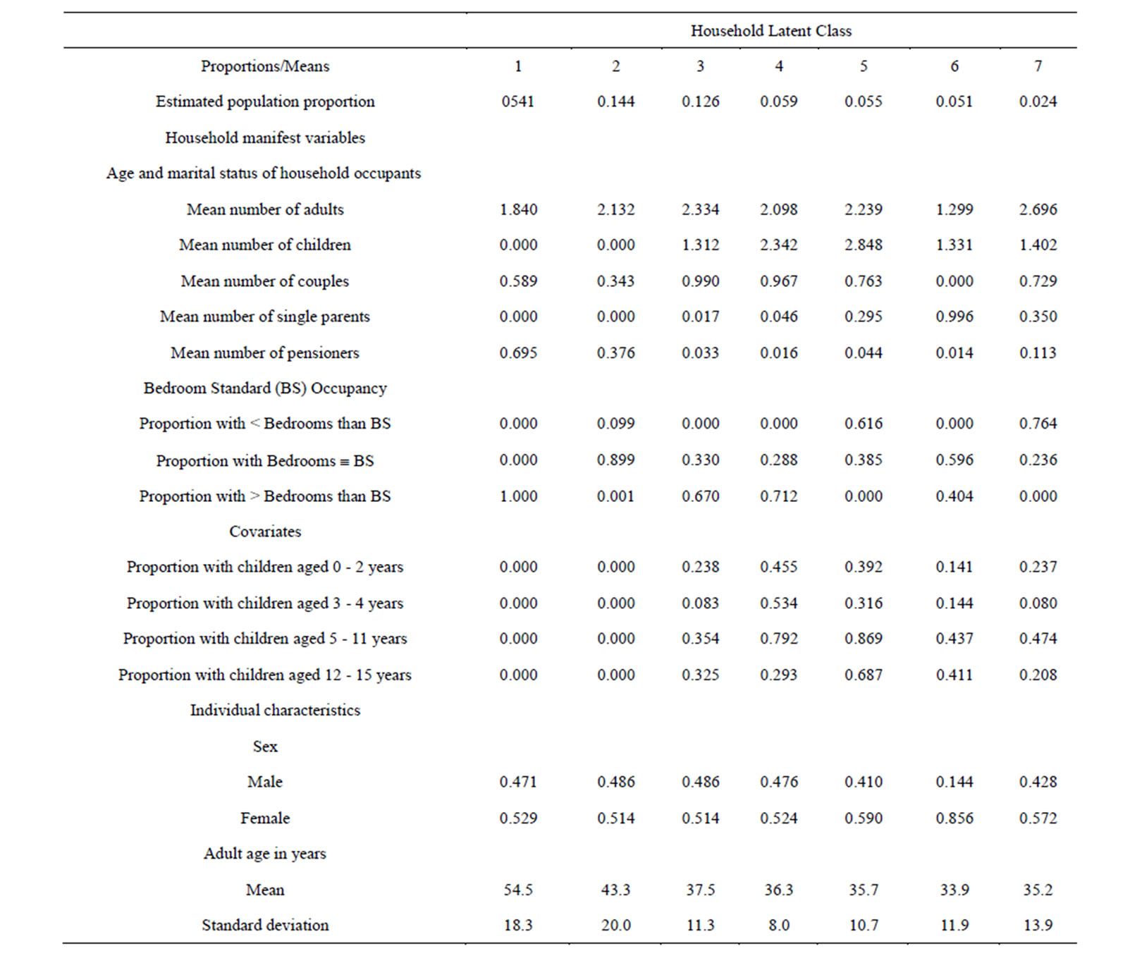
Table 4. Household manifest variables, covariates and individual characteristics of the seven latent household composition classes identified through LCA of Wave 2 USoc data (see Table 1) and labeled in Table 2.
minimum sufficient adjustment set.
As such this is the minimum sufficient adjustment set required for estimating the direct (as opposed to the total) effect of latent household composition class on sleep duration/quality. The largest latent household composition class (“Empty Nesters”) was then used as the reference group for comparison with each of the remaining household classes, since this class did not contain two ostensibly important household characteristics: neither children nor overcrowding. The results of these analyses have been summarized in Tables 5 and 6.
In terms of sleep duration (Table 5), these results indicate that, compared to adults living in households in the “Empty Nesters” class, adults in all of the remaining household classes had an increased risk of very short (i.e. <5 hrs) as opposed to 7 - 8 hrs sleep (the referent category). Adults in latent household composition classes with the highest risk of very short sleep duration included those living in classes labeled “Partnered with Children” (RR: 1.56; 95% CI: 1.29, 1.89) and “Large Family, Majority with Overcrowding” (RR: 1.57; 95% CI: 1.31, 1.88), adults living in the latter also having an increased risk (RR: 2.12; 95% CI: 1.54, 2.90) of very long (≥10 hrs) sleep duration.
In terms of sleep quality (Table 6), these results indicate that, compared to adults living in households in the “Empty Nesters” class, adults in all other household classes had an increased risk of “very bad” compared to

Table 5. Multinomial logistic regression exploring the relationship between latent household composition class and sleep duration, after adjustment for potential confounders1.

Table 6. Multinomial logistic regression exploring the relationship between latent household composition class and sleep quality, after adjustment for potential confounders1.
“fairly good” sleep. Adults in the latent household composition classes with the highest risk of having “very bad” sleep quality were those living in classes with overcrowding: “Extended Family, Majority with Overcrowding” (RR: 1.75; 95% CI: 1.34, 2.29) and “Large Family, Majority with Overcrowding” (RR: 1.51; 95% CI: 1.21, 1.87). Adults living in household classes with overcrowding also had an increased risk of “fairly bad” (versus “fairly good”) sleep quality, although those living in the “Single Parent Household” class (RR: 1.24; 95% CI: 1.08, 1.41) and the “Partnered with Children” class (RR: 1.24; 95% CI: 1.10, 1.4) had the highest relative risks in this category. Adults living in both the “Partnered with Children” class and the “Partnered with Child” class also had a reduced risk of “very good” versus “fairly good” sleep quality (RR: 0.85; 95% CI: 0.76, 0.95, and RR:0.88; 95% CI: 0.81, 0.95, respectively), indicating the importance of children in the household as a predictor of better than “fairly good sleep”.
3.3. Limitations
The data and analytical techniques used in the present study are subject to four key limitations, namely: a high prevalence of missing data for some of the key variables; variation in the numbers of respondents in different latent household composition classes; the somewhat subjective and limited acuity of latent class analysis (LCA); and incomplete adjustment for potential confounders in the relationship between latent household composition class and sleep duration/quality.
Despite the gift vouchers offered to USoc participants (and the separate risk this entails of participation bias), a substantial proportion of data were missing for many of variables included in the analyses. This was most pronounced for self-reported sleep duration and sleep quality, and as such the multinomial logistic regression analyses exploring the relationship between latent household composition class and sleep duration/quality (Tables 5 and 6) were conducted on a small subset of those respondents for whom data on sociodemographic and overcrowding data were available for the LCA summarized in Tables 1-3. Thus, while we are confident that the latent household composition classes identified from our analysis of the nationally representative USoc data are likely to reflect the distribution of these classes for the data set (and therefore the UK) as a whole, any tendency for differential reporting of sleep duration/quality by respondents from each of these household composition classes may undermine the strength and validity of their relationships with sleep (as summarized in Tables 5 and 6).
Indeed, the relatively small numbers of respondents in some of the latent household composition classes (particularly those containing children), will have inevitably reduced the statistical power of any relationship between these classes and self-reported sleep duration/quality. However, without conducting additional data collection to create boosted samples of respondents of all but those in the so-called “Empty Nesters” class, there was still more than a thousand (n = 1024; see Table 2), adult respondents in the class with the least respondents (the socalled “Extended Family, Majority with Overcrowding” class); and this sample size should have been more than sufficient to reveal any statistical association between household class and sleep duration/quality, even after the loss of respondents with missing data and the reduction in power incurred by adjustment for six potential confounders.
The choice of latent variable analysis used is therefore, perhaps, a more important potential limitation facing the present study. Although LCA is ostensibly an appropriate choice for classifying household composition, the categorization involved is essentially subjective. In particular, it was necessary to interpret means of count data (such as “1.84 adults”) to derive conceptually plausible labels for each of the latent classes—a process that is inherently subjective.
Using the Bayesian Information Criterion to establish which of the LCA models had the best statistical fit ensured that perhaps the most important aspects of this approach (that is, the number of latent household composition classes recognized as distinct) was data driven and determined by an objective statistical criterion. And since the results of the LCA models conducted on Wave 1 USoc data were very similar to those generated by LCA of Wave 2 data (see Table 4), we are confident that the approach we adopted successfully identified the (seven) most discrete, and therefore most important, latent household composition classes that could be described with the sociodemographic and overcrowding variables used. As for the labeling of these classes (e.g. as “Empty Nesters” or “Single Parent Household”), we offer these labels less as specific conceptual constructs per se and more as descriptive “handles” or monicker to facilitate the presentation, discussion and interpretation of the analyses.
Finally, the potential for under adjustment in the multinomial logistic regression analyses of the relationship between latent household composition class and sleep duration/quality (i.e. Tables 5 and 6) is a problem faced by any analysis of pre-existing observational data. This is because only those variables collected by the study (in this instance Wave 1 of USoc) are available for consideration/inclusion as potential confounders. Indeed, even when data are collected prospectively a decision will always have to make regarding which variables can and should be collected and which can/should not.
The importance of age, sex and social class as likely confounders in any relationship between living conditions (in this instance, household composition) and health (in this instance, sleep duration/quality) is what drove the selection of these variables (with highest educational attainment and ethnicity as proxies for the consequences/determinants of social class) as key potential confounders in these analyses. As such, we are confident that these analyses will have captured a substantial amount of the potential confounding linking latent household composition class and sleep duration/quality. Moreover, adjustment for two additional variables in these analyses (marital status and self-reported health) considered to be independent of household composition yet determinants of sleep duration/quality (i.e. considered “competing exposures” for sleep duration/quality), is likely to have improved the precision of any observed relationship between latent household composition class and the residual variation in sleep duration/quality. For these reasons, we are confident that the analyses described in Tables 5 and 6 provide a robust statistical assessment of these relationships.
3.4. Implications
Notwithstanding the limitations discussed above, the findings of the present study demonstrate the importance of considering potential inter-relationships between sociodemographic characteristics and overcrowding to operationalise the full complexity of household composition in large-scale epidemiological studies, such as USoc. Moreover, the study demonstrates that latent class analysis is capable of capturing a substantial proportion of this underlying complexity, generating distinct classes of household composition that are conceptually meaningful and statistically reliable/stable over time.
This is not only an important finding in its own right, but also has bearing on epidemiological analyses of outcomes that are likely to be household context-specific, such as a whole range of what might be considered “household lifestyle variables” including diet, activity and sleep. This is evident from the subtle yet important differences in self-reported adult sleep duration/quality observed amongst different latent household composition classes. These differences suggest that adults from household classes that are overcrowded or have children present report/experience shorter sleep durations and worse (or less good) sleep quality than those without overcrowding or children. Our study was also found some evidence that adults from household classes with both overcrowding and children (particularly two or more) reported the shortest sleep duration and worst (or least good) sleep quality—evidence that suggests the possibility of an interactive and/or summative effect of overcrowding and children on adult sleep patterns within households.
The results therefore indicate that adult sleep duration and quality are influenced by living in overcrowded homes and living with children, and suggest that not only the presence but also the number of children in the household plays a key role in the self-reported sleep of adults. For example, the “Partnered with Children” class had a higher risk of short sleep and “very bad” sleep quality than the “Partnered with Child” class–the main difference between these classes being that the former had at least one more additional child. This concurs with Chapman et al.’s [2] finding that the frequency of “insufficient sleep” was highest in households with 3 children. However, Groeger et al. [3] found that partnered adults with children had worse sleep duration and sleep quality outcomes than those adults in their study who belonged to the “Single Parent Household” class, the majority of whom (87.2%) were female.
This somewhat counterintuitive finding is perplexing, not least because women tend to report shorter and worse quality sleep than men (something we also observed, albeit incidentally, in our analysis of USoc data). Notwithstanding substantial differences in study design and context, one more straightforward possibility is that, in contrast to the sleep of unpartnered adults with children (which can only be influenced by their children and not by a non-existent adult partner), the sleep of partnered adults with children can be influenced not only by their children but also by their adult partner (and so on, by the impact of their children on their adult partner’s sleep).
Clearly, further research is warranted to quantify the relative importance of overcrowding, children and the number of children on adult sleep duration and quality, not least because overcrowded households are commonly those with one or more children. This is particularly important given the growing interest in and use of household occupancy measures (such as the UK’s Bedroom Standard) to determine overcrowding and welfare entitlements; and evidence linking appropriate levels of sleep duration and sleep quality as important prerequisites for mental and physical health.
ACKNOWLEDGEMENTS
Understanding Society is an initiative by the Economic and Social Research Council, with scientific leadership by the Institute for Social and Economic Research, University of Essex, and survey delivery by the National Centre for Social Research.
APPENDIX
DAGitty.net code to generate the DAG used to inform the analyses conducted in the present study. To view the DAG and its related minimum sufficient dataset, the text below can be pasted into the “model text data” window of www.dagitty.net:
Age 1 @-1.037, 1.268 Education 1 @-0.192, 1.236 Ethnicity 1 @-1.571, -2.098 Health 1 @1.238, 0.648 Household Class E @0.595, -0.431 Marital Status 1 @0.053, -2.079 Sex 1 @-1.554, -0.632 Sleep Duration %2F Quality O @1.420, -0.825 Age Household Class Sleep Duration %2F Quality Marital Status Education Health Education Household Class Sleep Duration %2F Quality Marital Status Health Ethnicity Household Class Sleep Duration %2F Quality Age Marital Status Education Health Health SleepDuration%2FQuality Household Class Sleep Duration %2F Quality Health Marital Status Household Class Sleep Duration %2F Quality Health
NOTES