Direct Numerical Simulation of a Jet Issuing from Rectangular Nozzle by the Vortex in Cell Method ()
1. Introduction
Vortex in cell (VIC) method [1] is one of the simulation methods for incompressible flows. It discretizes the vorticity field into vortex elements and computes the time evolution of the field by tracing the convection of each vortex element using the Lagrangian approach. The Lagrangian calculation markedly reduces numerical diffusion and also improves numerical stability. Thus, the VIC method is eminently suitable for direct numerical simulation (DNS) and large eddy simulation (LES) of turbulent flows, and various results have been reported. Cottet and Poncet [2] applied the VIC method for the wake simulation of a circular cylinder, and captured the streamwise vortices occurring behind the cylinder. Cocle et al. [3] analyzed the behavior of two vortex systems near a solid wall, and made clear the interaction between two counter-rotating vortices and the eddies induced in the vicinity of the wall. Chatelain et al. [4] simulated trailing edge vortices, and visualized the unsteady phenomena caused by disturbances. These studies are concerned with time-developing free shear flows. But the VIC method has not been applied to turbulent flows bounded by solid walls, which are closely related with the turbulent friction and heat transfer.
The authors [5] performed the DNS of a turbulent channel flow, which is a representative example of wall turbulent flows. When applying the existing VIC method, the oscillation of the flow increased with the progress of the computation, and eventually the computation collapsed. This was caused by the fact that the consistency among the discretized equations is not ensured. This was also because the solenoidal condition for the vorticity is not fully satisfied. To overcome such problems of the existing VIC method, the authors [5] proposed the improved VIC method. The authors [5] also applied the improved VIC method to the DNS of the turbulent channel flow. The DNS highlighted that the time evolution of the flow is fully computed and that the statistically steady turbulent flow is favorably obtained. It also demonstrated that the organized flow structures, such as streaks and streamwise vortices appearing in the near wall region, are successfully captured and that the turbulence statistics, such as the mean velocity and the Reynolds stress, agree well with the existing DNS results.
Jet is frequently observed in many engineering applications. As the jet is the representative of free shear flows governed by the convection of the eddies having various scales, the VIC method solving directly the vorticity field promises to be usefully applied to the simulation. But the VIC method has been scarcely used for the jet simulation.
The objective of this study is to search for the applicability of the authors’ VIC method [5] to the DNS of jet flows. The DNS of a jet issuing from a nozzle having a rectangular cross-section is performed by the VIC method. The jet velocity field was experimentally investigated by Iio et al. [6]. The aspect ratio of the nozzle cross-section is 15, and the Reynolds number based on the shorter side length of the nozzle exit is 6700. The DNS results, such as the mean velocity and the turbulence intensity, are favorably compared with the measured ones. The behavior of the large-scale eddies as well as the development of the turbulent flow is also confirmed to agree with the measurement. These indicate that the authors’ VIC method is successfully employed for the DNS of rectangular jet.
2. Vortex in Cell Method
2.1. Vorticity Equation and Orthogonal Decomposition of Velocity
For an incompressible flow, the vorticity equation is given by
 (1)
(1)
where u is the velocity and  is the vorticity.
According to the Helmholtz theorem, the velocity  is the sum of the curl of a vector potential
  and the gradient of a scalar potential
 :
:
 (2)
(2)
when  is postulated to be solenoidal or
 , the curl of Equation (2) yields the vector Poisson equation for
 :
:
 (3)
(3)
Substituting Equation (2) into the continuity equation and rewriting the resultant equation, the Laplace equation for  is obtained:
 (4)
(4)
Once  and
and  have been computed from Equations (3) and (4) respectively, the velocity
  is calculated from Equation (2). The vorticity
  in Equation (3) is estimated from Equation (1). The vortex in cell (VIC) method discretizes the vorticity field into vortex elements, and calculates the distribution of
  by tracing the convection of each vortex element.
It is postulated that the position vector and vorticity for the vortex element p are  and
and respectively. The Lagrangian form of the vorticity equation, Equation (1), is written as [7]:
 (5)
(5)
 (6)
(6)
When the position and vorticity of a vortex element are known at time , the values at
  are computed from the Lagrangian calculations of Equations (5) and (6). In the VIC method, the flow field is divided into computational grid cells to define
 ,
,  and
and  on the grids. If
  is defined at a position
 , the vorticity
  is assigned to
 , or a vortex element with vorticity
  is redistributed onto
 (7)
(7)
where ,
,  and
and  are the grid widths, and
  is the number of vortex elements. For the redistribution function
 , various forms are presented [7]. To suppress the numerical dissipation, a high-order scheme, which preserves the three first moments of the distribution, twice continuously differentiable and symmetric, is employed for
 :
:
 (8)
(8)
Equation (8) was used for the simulations of time-developing free shear flows [2-4]. The DNS of a turbulent channel flow was also successfully performed with Equation (8) by the authors [5].
2.2. Discretization by Staggered Grid
For incompressible flow simulations, the MAC and SMAC methods solve the Poisson equation, which is derived from the equation for pressure gradient and the continuity equation. These methods employ a staggered grid to ensure consistency among the discretized equations, and to prevent the numerical oscillation of the solution. The staggered grid would appear to be indispensable for discretizing the Poisson equation for  and the Laplace equation for
 , which are derived in the VIC method. However, staggered grids are not readily accommodated in the existing VIC method.
The authors proposed a VIC method using a staggered grid in their prior study [5]. Figure 1 shows the arrangement of the variables in the grid. The scalar potential  and velocity
  are defined at the center and sides of a grid cell, respectively. The vorticity
  and the vector potential
  are defined on the edges.
2.3. Correction of Vorticity Field
In the VIC method, the vorticity field is discretized into vortex elements, and the field is expressed by superimposing the vorticity distributions around each vortex element. The superposition is performed by Equation (7). The resulting vorticity field  does not necessarily satisfy the solenoidal condition [7]. Denoting the vorticity satisfying this condition by
 ,
,  is represented as [3]
 (9)
(9)
where F is a scalar function. Equation (9) corresponds to the Helmholtz decomposition of .
.
Taking the divergence of Equation (9), the Poisson equation for F is obtained:
 (10)
(10)
Calculating F from Equation (10) and substituting into Equation (9) gives the recalculated vorticity  [3]. This correction for vorticity needs to solve the Poisson equation, which increases the computational time. To reduce this additional cost, the authors [5] have proposed a simplified correction method.
The uncorrected vorticity,  , is linked to
  through Equation (3). Taking the divergence of Equation (3) and substituting Equation (10) into the resultant equation, the following relations are obtained:
 (11)
(11)
Unlike the assumption for the solenoidal condition of , the following equation for a non-solenoidal vorticity is derived from Equation (11).
 (12)
(12)
Using  to calculate
  from Equation (3), and determining
  from Equation (4), the curl of
  transforms as follows:
 (13)
(13)
Equation (13) demonstrates that the curl of the velocity  calculated from
  yields a vorticity
  that satisfies the solenoidal condition. If the vorticity is recalculated by Equation (13), or the vorticity is corrected immediately after calculating the velocity by Equation (2), the discretization error in the vorticity is completely removed and the flow dynamics are accurately simulated without solving the Poisson equation, Equation (10). It should be noted that the staggered grid is required for rendering the transformation in Equation (13) applicable to the corresponding discretized equations.
2.4. Simulation Procedure
Given the flow at time , the flow at
  is simulated by the following procedure:
1) Calculate the change in the strength of each vortex element defined on the grid, or calculate the vorticity  from Equation (6).
2) Calculate the convection of each vortex element, or calculate the position  from Equation (5).
3) Redistribute the vortex element onto the grids, or calculate the vorticity  on the grids by Equation (7).
4) Calculate the vector potential  from Equation (3).
5) Calculate the scalar potential  from Equation (4).
6) Calculate the velocity  from Equation (2).
7) Correct the vorticity, or calculate the corrected vorticity from the curl of .
.
3. Simulation Conditions
The DNS of an incompressible jet issuing from a nozzle having a rectangular cross-section is performed. The jet velocity field was experimentally investigated by Iio et al. [6]. The computational domain is shown in Figure 2. The shorter side length of the nozzle exit is , and the longer side length is
 . The
. The  -axis is along the jet centerline, while the
  - and
- and  -axes are parallel to the shorter and longer sides of the nozzle exit respectively. The computational domain consists of a cubic region of
 . It is resolved into uniform grid cells of
 . Consequently, the shorter and longer sides of the nozzle exit are divided by 10 and 150 cells

Figure 2. Rectangular nozzle and computational domain.
respectively. The jet velocity at the nozzle exit is , and the Reynolds number based on
  and
and  is 6700. Table 1 summarizes the simulation conditions.
The boundary conditions are given as follows: Within the nozzle exit, a uniform and constant velocity  is imposed.
 (14)
(14)
The non-slip condition is adopted on the wall at , on which the nozzle exit is mounted.
 (15)
(15)
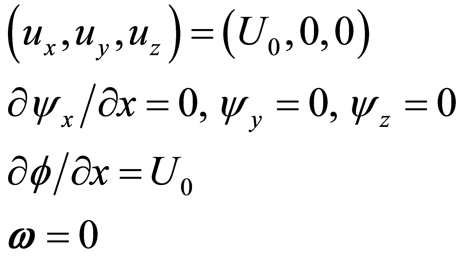
The velocity gradient is set at zero on the other boundaries. For example, the following conditions are imposed at .
.
 (16)
(16)
The time increment  is
is . A fully developed flow was obtained at a time of
 . The time-averaged velocity and the turbulence intensity were acquired in the period from
  to
to .
.
4. Results and Discussion
4.1. Instantaneous Flow Fields
The instantaneous distribution for the absolute value of
the velocity  for the fully developed jet is shown in Figure 3. The distribution on the central cross-sections of the jet is presented. Figure 3(a) shows the result on the x-y cross-section at z = 0 parallel to the shorter side of the nozzle exit. The potential core disappears at x/w ≒ 2.6, as mentioned later. Thus, the jet spreads in the lateral direction downstream of the disappearing point, indicating the momentum diffusion in the direction. The distribution on the x-z cross-section parallel to the longer side is shown in Figure 3(b). It should be noted that the jet width becomes slightly narrower as the streamwise distance increases.
The vorticity components  and
and  at the same instant as Figure 3 distribute as plotted in Figure 4, where the distributions on the jet central cross-sections are presented. The shear layers originate from the shorter and longer sides of the nozzle exit, and the turbulent flow rapidly develops just after the collapse of the shear layers.
Figure 5(a) shows the velocity on the jet central crosssection parallel to the shorter side of the nozzle exit, where the distribution near the nozzle is plotted. To make the distribution more understandable, the velocity  is subtracted. On the shear layers originating from the longer sides of the nozzle exit, large-scale eddies occur at x/w ≧ 2.2. The eddies are non-axisymmetric around the jet centerline. They change into eddies having various scales as the streamwise distance increases. Figure 5(b) presents the flow field visualized experimentally by illuminating an alcohol mist with a laser light sheet [6]. The image clearly visualizes the occurrence of some largescale eddies on the shear layers as well as the rapid change of the flow into turbulence. It is confirmed that the DNS successfully resolves the flow development including the occurrence and collapse of large-scale eddies.